1 Outlook
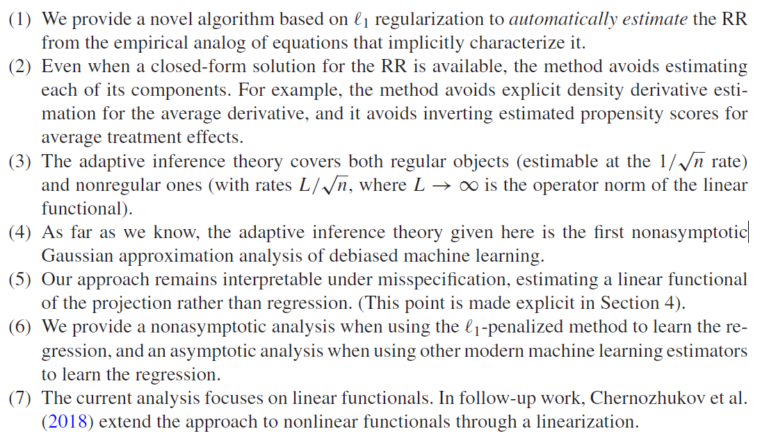
- \ell_1-based inference for regular/global (semiparametric) and irregular/local (nonparametric) linear functionals of the conditional expectation function
- Regular examples: ATE, derivatives, \ldots
- Irregular examples: Conditional ATE etc. fixed at a specific point
- Framework utilizes Neyman Orthogonality which is based on Riesz Representer (RR) (which is estimated as a nuisance parameter); connection to double robustness
- \ell_1-based inference: Either outcome regression or RR can be dense if other part is sufficiently sparse
- Non-asymptotic results and implication of asymptotic uniformly validity \Rightarrow honest confidence bands for global and local parameters
2 Introduction
Many statistical objects of interest can be expressed as a linear functional of a regression function (or projection, more generally).
Central problem here: Inference on linear functionals of regressions (sounds abstract, see Section 2.1).
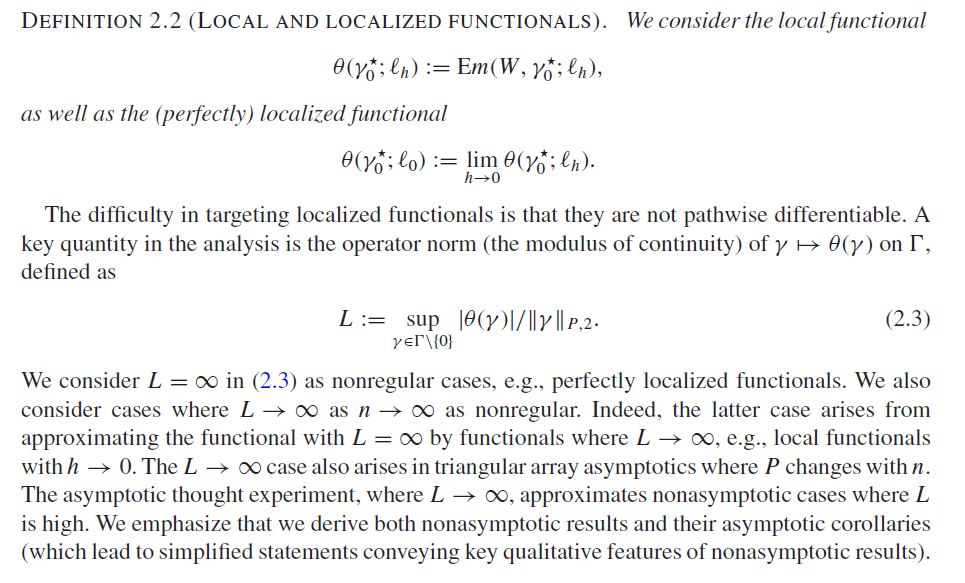
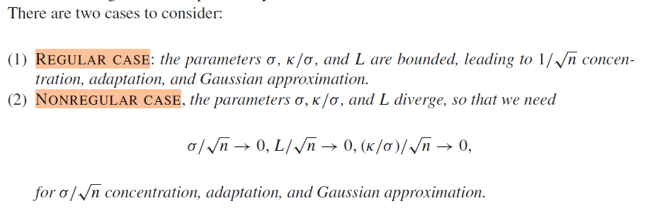
- Global parameters are typically regular (1/\sqrt{N} rate)
- Local parameters are typically irregular (slower than 1/\sqrt{N} rate)
Here: One inferential framework covering both regular and irregular estimands
Use of ML for inference: Double Machine Learning
- “Double” because of double robustness - property of orthogonal scores
Scores are constructed by adding bias correction term: The average product of the regression residual with a learner of the functional’s Riesz representer
\begin{equation*} \theta ^\star _0 = \theta (\alpha _0^\star ,\gamma _0^\star ); \ \ \theta (\alpha , \gamma ) := {\mathrm{E}}[m(W, \gamma ) + \alpha (X) (Y - \gamma (X))], \end{equation*}
- Advantages of approach
2.1 Motivation Example: Riesz representer
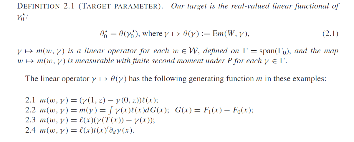
- Average Treatment Effect (ATE)1

ATE: \begin{align*} m(\omega, \gamma) &= \gamma(1,Z) - \gamma(0,Z)\\ &= E[Y|D=1,Z] - E[Y|D=0,Z] \end{align*}
ATE: Riesz-representer = Horvitz-Thomson Transform (Inverse Propensity Score Weighting) \alpha_0(Z) = \frac{D}{\pi(Z)} - \frac{1-D}{1-\pi(Z)}
3 Ways of estimation
- Direct Plug-in Estimator (Regression)
- Imposing specification for \gamma
- Inverse- Propensity Score weighting & plugging-in empirical analogs
- Imposing specification for \alpha / prop. score & plugging-in empirical analogs
- Doubly robust
- Tolerating misspecification through double robustness property
- Direct Plug-in Estimator (Regression)
3 Framework and Target Parameters
3.1 Setup
\ldots [Some notation and assumptions]
Unknown regression function (later being replaced by a projection in general part) x \mapsto \gamma^*_0(x) \coloneqq E[Y|X=x]
\Gamma_0 convex parameter space for \gamma^* with elements \gamma
Goal: High quality inference for real-valued linear functionals of \gamma^*_0.
Using causal assumptions for interpretation/examples
- Exogeneity/Unconfoundedness
Examples for target parameters
- [W]ATE (ATE, ATET, GATEs, using differen weighting functions \ell(x)) (see Section 2.1)
- Effect from changing distribution of X
- Effect from transporting X
- Average directional derivative
1.-4. all have the interpretation as real-valued linear functions of the regression function & therefore share a common structure for inference
- Estimation is straightforward if weights are known (e.g. Horvitz-Thompson estimator)
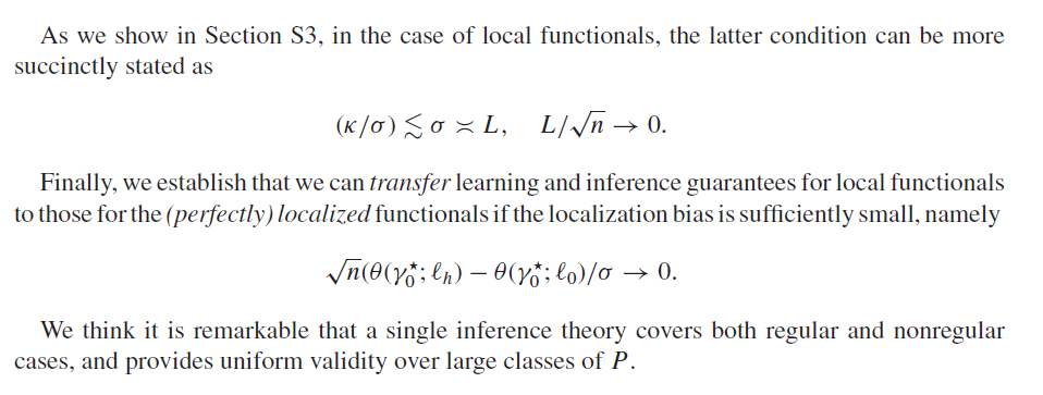
3.2 Local and Localized Functionals
3.3 Orthogonality
3.3.1 Definition: Linear and Minimal Linear Representer

- A minimal linear representer exists if and only if L < \infty
3.3.2 Non-orthogonality

3.3.3 Orthogonal representation
\begin{equation*} \theta ^\star _0 = \theta (\alpha _0^\star ,\gamma _0^\star ); \ \ \theta (\alpha , \gamma ) := {\mathrm{E}}[m(W, \gamma ) + \alpha (X) (Y - \gamma (X))], \end{equation*} where (\alpha, \gamma) are the nuisance parameters with true value (\alpha^*, \gamma^*).
Unlike the direct or dual representations for the functional, this representation is Neyman orthogonal to perturbations (\bar{h}, h)\in \Sigma^2 of (\alpha^*, \gamma^*) s.t. \begin{equation*} \frac{\partial }{\partial t} \theta (\alpha _0^\star + t \bar{h}, \gamma _0^\star + t h) \Big |_{t=0} = {\mathrm{E}}m(W, h) - {\mathrm{E}}\alpha _0^\star (X) h(X) + {\mathrm{E}}[(Y - \gamma _0^\star (X)) \bar{h}(X)] = 0.\end{equation*}
Even a stronger property holds \begin{equation*} \theta (\alpha , \gamma ) - \theta (\alpha ^\star _0, \gamma ^\star _0) = - \int (\gamma - \gamma ^\star _0) ( \alpha - \alpha _0^\star ) dF, \end{equation*} which implies Neyman orthogonality as well as double robustness
The Neyman orthogonality property states that the representation of the target parameter \theta_0 in terms of the nuisance parameters (\alpha, \gamma) is invariant to the local perturbations of the values of the nuisance parameter
3.3.4 Finite-dimensional regression

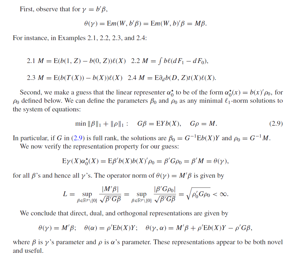
3.3.5 Infinite-dimensional regression

Estimation result relies on existence of minimal representers
Minimal representers also important for efficiency
3.3.6 Informal preview / Algorithm
Estimation and inference based on orthogonal representation and equation for Riesz representer
(\theta(\gamma) = E[\gamma(X) \alpha_0(X)], \forall \gamma \in \Gamma)General idea:
- Approximate \alpha^*_0 by linear form b'\rho_0
- Approximate \gamma^*_0 by projection b'\beta_0
- Use cross-fitting and estimate coefficients by \ell_1-penalized regression (Generalized Dantzig selector, some generaliztion to generic estimation of \hat\gamma possible, see Section 5)
- Target coefficient obtained from empirical analog of orthogonal score
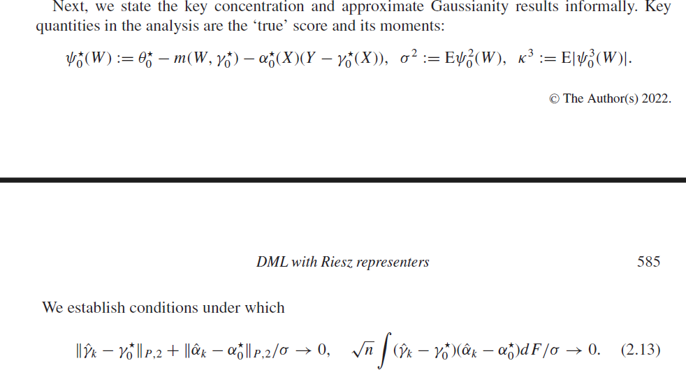
Conditions: Bound on \ell_1-norm of coefficients and sparsity of either RR or regression function, effective dimension s less than \sqrt(N)
If (2.13) holds, then DML estimator is adaptive: approximated up to the error o(\sigma/\sqrt{N}) by oracle estimator2 \begin{equation*} \bar{\theta }:= \theta ^\star _0 - n^{-1} \sum _{i =1}^n \psi _0(W_i), \end{equation*}
Approximation deviation of \hat{\theta} from \theta^*_0 is determined by ||\psi_0||_{P,2}/\sqrt{N} (=standard deviation)
Hence: \theta^*_0 concentrates in \sigma/\sqrt{N}-neighborhood of the target (normality)

4 Infinite Dimensions
See paper
