Sensitivity Analysis for Causal ML:
A Use Case at Booking.com

Philipp Bach, Victor Chernozhukov, Carlos Cinelli, Lin Jia, Sven Klaassen, Nils Skotara, Martin Spindler

KDD Barcelona, Causal Inference & ML in Practice Workshop
August 26, 2024
University of Hamburg, MIT, University of Washington, Booking.com, Economic AI

Outline

Motivation: Sensitivity Analysis & Use Case

Estimand of Interest: ATT

Sensitivity Analysis in a Use Case at Booking.com

Summary and Outlook

Motivation: Sensitivity Analysis & Use Case

Sensitivity Analysis

• Causal inference is inherently based on untestable assumptions

• Standard assumption in observational studies
  Unconfoundedness: Treatment assignment is independent of potential outcomes given covariates (see details here)

• 😱 Assumption might be very strong and difficult to justify in practice (unobserved confounding)

➡️ Sensitivity analysis as a tool to establish trust in our estimates

🤔 How much can we trust our estimates when it is violated?

import networkx as nx
import matplotlib.pyplot as plt

G = nx.DiGraph()

# Add nodes
G.add_node("D")
G.add_node("Y")
G.add_node("X")
G.add_node("U")
G.add_edge("D", "Y")
G.add_edge("X", "Y")
G.add_edge("X", "D")
G.add_edge("U", "D")
G.add_edge("U", "Y")

# Draw the graph
plt.figure(figsize=(4, 3)) 
pos = {"D": (0, 0), "Y": (2, 0), "X": (1,1), "U": (1,-1)}
edge_colors = ['black', 'black', 'black', 'red', 'blue']
nx.draw(G, pos, with_labels=True, node_size=800, node_color='lightblue',
 edge_color=edge_colors)
plt.show()

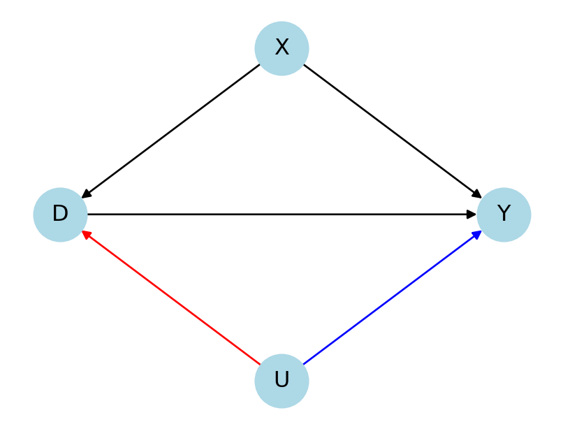
DAG: Causal Effect of D on Y, with observed confounders X and unobserved confounders U.

Motivation: Sensitivity Analysis & Use Case

Use Case

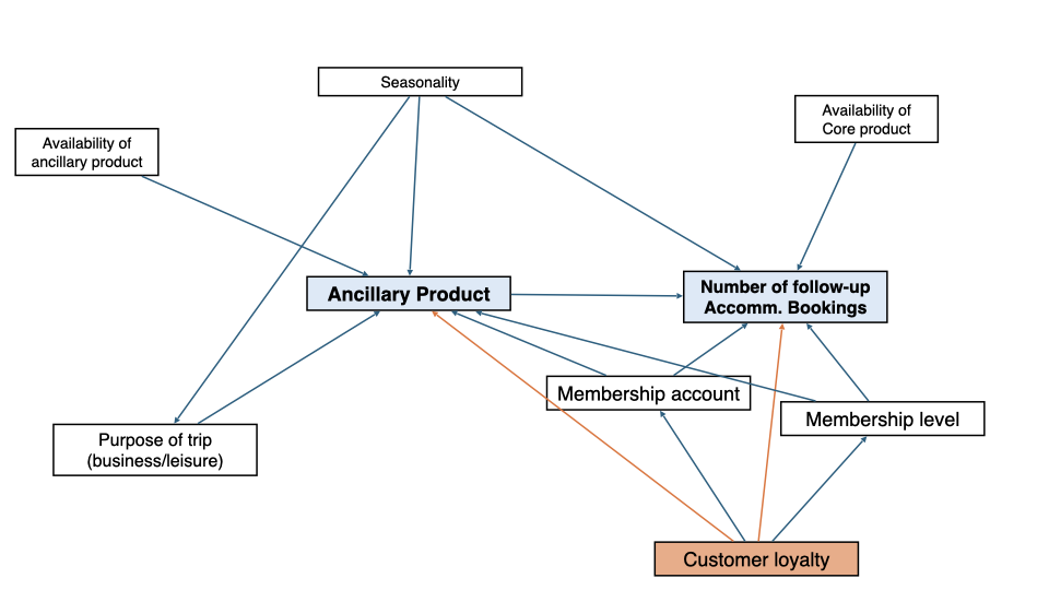
• Key question: What is the causal effect of purchasing an ancillary product (taxi transfer, flight, etc.) on follow-up bookings?

• Analysis based on observational data (past transactions)

• Major concern: Unmodelled customer loyalty might affect users’ propensity to purchase ancillary products and to make follow-up bookings ➡️ Upward bias

Stylized DAG from use case at Booking.com.

The presented results are based on a simulated data set and cannot be used to recover the findings from the actual use case at Booking.com . Replicable notebook available at https://docs.doubleml.org/stable/examples/py_double_ml_sensitivity_booking.html.

Estimand of Interest: ATT

Average Treatment Effect on the Treated (ATT)

\[ \theta_0 = \mathbb{E}[Y(1) \mid D=1]- \mathbb{E}[Y(0) \mid D=1]. \]

• ATT measures the average impact on follow-up bookings that results from booking an ancillary product

• The ATT can be identified under the assumption of unconfoundedness (see details here)

• Sensitivity analysis based on Chernozhukov et al. (2022) and implemented in DoubleML for Python (Bach et al. 2022)

Estimand of Interest: ATT

Sensitivity Analysis (Chernozhukov et al. 2022)

• Long parameter (if we had access to the unobserved confounder(s))

\[ \theta_0 = \mathbb{E}[Y|D=1] - \mathbb{E}[\mathbb{E}[Y|D=0, X, U]|D=1]. \]

• Short parameter (only observed data)

\[ \theta_s = \mathbb{E}[Y|D=1] - \mathbb{E}[\mathbb{E}[Y|D=0, X]|D=1]. \]

• Omitted variable / confounding bias:

\[\text{bias} = |\theta_s - \theta_0|\]

Estimand of Interest: ATT

Sensitivity Analysis (Chernozhukov et al. 2022)

• Idea of sensitivity analysis: Parametrize confounding in terms of sensitivity parameters and assess confounding bias in different scenarios

• Extensive literature from statistics, econometrics and computer science (see References)

• Chernozhukov et al. (2022): Formula for omitted variable bias in very general framework, based on Riesz Representation (Chernozhukov, Newey, and Singh 2022) for ATT, see more details here

\[ \text{bias}^2 = \rho^2 C_Y^2 C_D^2 S^2. \]

import networkx as nx
import matplotlib.pyplot as plt

G = nx.DiGraph()

# Add nodes
G.add_node("D")
G.add_node("Y")
G.add_node("X")
G.add_node("U")
G.add_edge("D", "Y")
G.add_edge("X", "Y")
G.add_edge("X", "D")
G.add_edge("U", "D")
G.add_edge("U", "Y")

# Draw the graph
plt.figure(figsize=(4, 3)) 
pos = {"D": (0, 0), "Y": (2, 0), "X": (1,1), "U": (1,-1)}
edge_colors = ['black', 'black', 'black', 'red', 'blue']
nx.draw(G, pos, with_labels=True, node_size=800, node_color='lightblue',
 edge_color=edge_colors)
plt.show()

DAG: Causal Effect of D on Y, with observed confounders X and unobserved confounders U.

Estimand of Interest: ATT

Sensitivity Parameters (Chernozhukov et al. 2022)

• \(S^2\): Scaling factor that can be estimated from the data

• \(\rho^2\): Correlation of the confounding variation in terms of the outcome variable and the treatment variable, respectively

• \(C_Y^2\): (Nonparametric) partial \(R^2\) of \(U\) with respect to \(Y\)

\[ \begin{align} C_Y^2 & := \frac{\text{Var}(\mathbb{E}[Y \mid D, X, U]) - \text{Var}(\mathbb{E}[Y \mid D, X])}{\text{Var}(Y) - \text{Var}(\mathbb{E}[Y \mid D, X])} \\ & := R^2_Y \end{align} \]

Estimand of Interest: ATT

Sensitivity Parameters (Chernozhukov et al. 2022)

• \(C_D^2\): Increase in the average odds of receiving treatment due to the presence of the unobserved confounder \(U\)

\[ \begin{align*} C_D^2 = \frac{\mathbb{E}\left[O(X, U)\right] - \mathbb{E}\left[O(X)\right]}{\mathbb{E}\left[O(X)\right]}, \end{align*} \] with odd ratios \[O(X, U) := \frac{P(D=1 \mid X, U)}{1 - P(D=1 \mid X, U)},\] and \[O(X) := \frac{P(D=1 \mid X)}{1 - P(D=1 \mid X)}. \]

Estimand of Interest: ATT

Sensitivity Parameters (Chernozhukov et al. 2022)

• Implementation and results are based on a rescaled version that is bounded to \([0,1)\)

\[C_D^2 = \frac{R^2_D}{1 - R^2_D},\] such that

\[ \begin{align} R^2_D := & \frac{\mathbb{E}\left[O(X, U)\right] - \mathbb{E}\left[O(X)\right]}{\mathbb{E}\left[O(X, U)\right]}. \end{align} \]

Estimand of Interest: ATT

Outlook: Type of results

• Given a confounding scenario that is parametrized in terms of \(C_Y^2\), \(C_D^2\) and \(\rho^2\), we can bound the omitted variable bias (see Chernozhukov et al. 2022 for more details)

However, how to get these scenarios?

1. Domain expertise
2. Benchmarking (omitting known confounders)

• Standard reporting, in particular if no specific scenarios can be formulated: Robustness values
  • \(RV\): Minimum symmetric confounding scenario that would suffice to explain away the reported estimate
  • \(RV_a\): Take sampling variance into account (significance)

Sensitivity Analysis in a Use Case at Booking.com

Estimation and Sensitivity Analysis

• Estimation based on Double Machine Learning (DML) (Chernozhukov et al. 2018), DoubleML for Python, using LightGBM learners

• Sample: Visitors of the Booking.com websites and users of app in a pre-specified window of 6 months

• Preliminary results: ATT estimate of \(0.123^{***}\), but robustness is questionable

Stylized DAG from use case at Booking.com.

Sensitivity Analysis in a Use Case at Booking.com

Estimation and Sensitivity Analysis

# Complete notebook available at https://docs.doubleml.org/stable/examples/py_double_ml_sensitivity_booking.html
import doubleml as dml
from doubleml.datasets import make_confounded_irm_data

import numpy as np
import pandas as pd
import matplotlib.pyplot as plt
import seaborn as sns

from sklearn.linear_model import LinearRegression, LogisticRegression
from sklearn.ensemble import RandomForestRegressor, RandomForestClassifier
from sklearn.isotonic import IsotonicRegression
from lightgbm import LGBMRegressor, LGBMClassifier
import plotly.graph_objects as go

# Use smaller number of observations in demo example to reduce computational time
n_obs = 75000

# Parameters for the data generating process
# True average treatment effect (very similar to ATT in this example)
theta = 0.07
# Coefficient of the unobserved confounder in the outcome regression.
beta_a = 0.25
# Coefficient of the unobserved confounder in the propensity score.
gamma_a = 0.123
# Variance for outcome regression error
var_eps = 1.5
# Threshold being applied on trimming propensity score on the population level
trimming_threshold = 0.05

# Number of observations
np.random.seed(42)
dgp_dict = make_confounded_irm_data(n_obs=n_obs, theta=theta, beta_a=beta_a, gamma_a=gamma_a, var_eps=var_eps, trimming_threshold=trimming_threshold)

x_cols = [f'X{i + 1}' for i in np.arange(dgp_dict['x'].shape[1])]
df = pd.DataFrame(np.column_stack((dgp_dict['x'], dgp_dict['y'], dgp_dict['d'])), columns=x_cols + ['y', 'd'])

# Set up the data backend with treatment variable d, outcome variable y, and covariates x
dml_data = dml.DoubleMLData(df, 'y', 'd', x_cols)

# Initialize LightGBM learners
n_estimators = 150
learning_rate = 0.05
ml_g = LGBMRegressor(n_estimators=n_estimators, learning_rate = 0.05, verbose=-1)
ml_m = LGBMClassifier(n_estimators=n_estimators, learning_rate = 0.05, verbose=-1)

# Initialize the DoubleMLIRM model, specify score "ATTE" for average treatment effect on the treated
dml_obj = dml.DoubleMLIRM(dml_data, score = "ATTE", ml_g = ml_g, ml_m = ml_m, n_folds = 5, n_rep = 2)


# fit the model
dml_obj.fit()

dml_obj.summary.round(3)

	coef	std err	t	P>|t|	2.5 %	97.5 %
d	0.123	0.008	15.065	0.0	0.107	0.139

Sensitivity Analysis in a Use Case at Booking.com

# Take values from preferred confounding scenario (based on benchmarking with respect to some of the membership variables)
cf_y=0.09187106073162674
cf_d=0.0028213335041910427
rho=1.0

# benchmarking scenario
dml_obj.sensitivity_analysis(cf_y = cf_y, cf_d = cf_d, rho = 1.0)
print(dml_obj.sensitivity_summary)

================== Sensitivity Analysis ==================

------------------ Scenario          ------------------
Significance Level: level=0.95
Sensitivity parameters: cf_y=0.09187106073162674; cf_d=0.0028213335041910427, rho=1.0

------------------ Bounds with CI    ------------------
   CI lower  theta lower     theta  theta upper  CI upper
0  0.073908      0.08736  0.123192     0.159025  0.172482

------------------ Robustness Values ------------------
   H_0    RV (%)   RVa (%)
0  0.0  5.391377  4.816176

• \(RV\): Unobserved confounders that explain less than \(7.579\%\) of the residual variation of the outcome and of the odds of treatment, are logically incapable of bringing the point estimate of the ATT to zero.

• \(RV_a\): If we consider sampling uncertainty, this number reduces to \(6.779\%\) (at the 5% significance level).

Sensitivity Analysis in a Use Case at Booking.com

# Sensitivity analysis with benchmark scenario for X2 (which is supposed to be "not unlike the omitted confounder")
contour_plot = dml_obj.sensitivity_plot(include_scenario=True, grid_bounds = (0.08, 0.12))

# Add robustness value to the plot: Intersection of diagonal with contour line at zero
rv = dml_obj.sensitivity_params['rv']

# Add the point with an "x" shape at coordinates (rv, rv)
contour_plot.add_trace(go.Scatter(
    x=rv,
    y=rv,
    mode='markers+text',
    marker=dict(
        size=12,
        symbol='x',
        color='white'
    ),
    name="RV",
    showlegend = False
))

# Set smaller margin for better visibility (for paper version of the plot)
contour_plot.update_layout(
    margin=dict(l=1, r=1, t=5, b=5)
)

contour_plot.show()

Summary and Outlook

Summary

• Discussions with domain experts and benchmarking scenarios point at a rather robust ATT estimate, although the preliminary estimate is probably biased upwards

• Sensitivity analysis was very useful to assess the robustness of the ATT estimate in the use case at Booking.com (standard step of causal workflow)

• Project helped to better understand the importance of identification and unobserved confounding, which is crucial in (observational) causal inference

• Link to domain experts was essential to define meaningful scenarios and to interpret the results

• Considerable impact on communication and decision-making processes (stakeholders, management); valuable insights for future research

Thank you!

Contact

In case you have questions or comments, feel free to contact us:

philipp.bach@uni-hamburg.de

Package Stickers

Get your DoubleML stickers after the talk 😃 & leave a 🌟 on GitHub: https://github.com/DoubleML/doubleml-for-py

Acknowledgement

DoubleML gratefully acknowledges support by Economic AI 🙏

Economic AI - Causal ML for Business Applications.

Appendix

Identification under Unconfoundedness

The ATT can be from the distribution of observed data \(W_s = (Y, D, X)\) under the following assumptions:

• Unconfoundedness: \(\{Y(0), Y(1)\} \perp\!\!\!\perp D \vert X\),

• Overlap: \(0 < P(D=1 \vert X) < 1\),

• Consistency: \(Y=Y(D)\).

Riesz Representation: ATT

We are interested in the causal parameter \(\theta_0\) that can be identified as a linear functional of the long regression function \(g_0:=\mathbb{E}[Y|D, X, U]\) \[ \begin{align*} \theta_0 = \mathbb{E}[m(W,g_0)], \end{align*} \] where \(m\) is a formula that is affine in \(g_0\), \(W\) denotes the full data vector, \(W= (Y, D, X, U)\).

Key idea: Express the long parameter \(\theta_0\) as the inner product of the long regression, and weights \(\alpha_0\), \[ \begin{align*} \theta_0 = \mathbb{E}[m(W, g_0)] = \mathbb{E}[g_0(W)\alpha_0(W)], \end{align*} \] where \(\alpha_0(W)\) is called the Riesz representer of \(\theta_0\).

Riesz Representation: ATT

• Riesz representers for the ATT

\[ \begin{align} \alpha_0(W) &= \left(\frac{D}{m_0(X, U)} - \frac{1-D}{1-m_0(X, U)}\right) \left(\frac{m_0(X, U)}{p}\right),\nonumber\\ \alpha_s(W_s) &= \left(\frac{D}{m_s(X)} - \frac{1-D}{1-m_s(X)}\right) \left(\frac{m_s(X)}{p}\right),\nonumber \end{align} \] where \(p := P(D=1)\).

• More details in paper and references therein.

References

References

Bach, Philipp, Victor Chernozhukov, Carlos Cinelli, Lin Jia, Sven Klaassen, Nils Skotara, and Martin Spindler. 2024. “Sensitivity Analysis for Causal ML: A Use Case at Booking.com.” In Proceedings of the KDD’24 Workshop on Causal Inference and Machine Learning in Practice.

Bach, Philipp, Victor Chernozhukov, Malte S Kurz, and Martin Spindler. 2022. “DoubleML-an Object-Oriented Implementation of Double Machine Learning in Python.” Journal of Machine Learning Research 23: 53–51.

Bach, Philipp, Malte S. Kurz, Victor Chernozhukov, Martin Spindler, and Sven Klaassen. 2024. “DoubleML: An Object-Oriented Implementation of Double Machine Learning in R.” Journal of Statistical Software. https://doi.org/10.18637/jss.v108.i03.

Blackwell, Matthew. 2013. “A Selection Bias Approach to Sensitivity Analysis for Causal Effects.” Political Analysis 22 (2): 169–82.

Brumback, Babette A, Miguel A Hernán, Sebastien JPA Haneuse, and James M Robins. 2004. “Sensitivity Analyses for Unmeasured Confounding Assuming a Marginal Structural Model for Repeated Measures.” Statistics in Medicine 23 (5): 749–67.

Carnegie, Nicole Bohme, Masataka Harada, and Jennifer L Hill. 2016. “Assessing Sensitivity to Unmeasured Confounding Using a Simulated Potential Confounder.” Journal of Research on Educational Effectiveness 9 (3): 395–420.

Chernozhukov, Victor, Denis Chetverikov, Mert Demirer, Esther Duflo, Christian Hansen, Whitney Newey, and James Robins. 2018. “Double/Debiased Machine Learning for Treatment and Structural Parameters.” The Econometrics Journal 21 (1): C1–68. https://onlinelibrary.wiley.com/doi/abs/10.1111/ectj.12097.

Chernozhukov, Victor, Carlos Cinelli, Whitney Newey, Amit Sharma, and Vasilis Syrgkanis. 2022. “Long Story Short: Omitted Variable Bias in Causal Machine Learning.” National Bureau of Economic Research. https://doi.org/10.48550/arXiv.2112.13398.

Chernozhukov, Victor, Christian Hansen, Nathan Kallus, Martin Spindler, and Vasilis Syrgkanis. forthcoming. Applied Causal Inference Powered by ML and AI. online. https://causalml-book.org/.

Chernozhukov, Victor, Whitney K Newey, and Rahul Singh. 2022. “Automatic Debiased Machine Learning of Causal and Structural Effects.” Econometrica 90 (3): 967–1027.

Cinelli, Carlos, Jeremy Ferwerda, and Chad Hazlett. 2020. “Sensemakr: Sensitivity Analysis Tools for OLS in r and Stata.” Available at SSRN 3588978.

Cinelli, Carlos, and Chad Hazlett. 2020. “Making Sense of Sensitivity: Extending Omitted Variable Bias.” Journal of the Royal Statistical Society Series B: Statistical Methodology 82 (1): 39–67.

———. 2022. “An Omitted Variable Bias Framework for Sensitivity Analysis of Instrumental Variables.” Available at SSRN 4217915.

Cinelli, Carlos, Daniel Kumor, Bryant Chen, Judea Pearl, and Elias Bareinboim. 2019. “Sensitivity Analysis of Linear Structural Causal Models.” International Conference on Machine Learning.

Cornfield, Jerome, William Haenszel, E Cuyler Hammond, Abraham M Lilienfeld, Michael B Shimkin, and Ernst L Wynder. 1959. “Smoking and Lung Cancer: Recent Evidence and a Discussion of Some Questions.” Journal of National Cancer Institute, no. 23: 173–203.

Dorie, Vincent, Masataka Harada, Nicole Bohme Carnegie, and Jennifer Hill. 2016. “A Flexible, Interpretable Framework for Assessing Sensitivity to Unmeasured Confounding.” Statistics in Medicine 35 (20): 3453–70.

Frank, Kenneth A. 2000. “Impact of a Confounding Variable on a Regression Coefficient.” Sociological Methods & Research 29 (2): 147–94.

Frank, Kenneth A, Spiro J Maroulis, Minh Q Duong, and Benjamin M Kelcey. 2013. “What Would It Take to Change an Inference? Using Rubin’s Causal Model to Interpret the Robustness of Causal Inferences.” Educational Evaluation and Policy Analysis 35 (4): 437–60.

Frank, Kenneth A, Gary Sykes, Dorothea Anagnostopoulos, Marisa Cannata, Linda Chard, Ann Krause, and Raven McCrory. 2008. “Does NBPTS Certification Affect the Number of Colleagues a Teacher Helps with Instructional Matters?” Educational Evaluation and Policy Analysis 30 (1): 3–30.

Hosman, Carrie A, Ben B Hansen, and Paul W Holland. 2010. “The Sensitivity of Linear Regression Coefficients’ Confidence Limits to the Omission of a Confounder.” The Annals of Applied Statistics, 849–70.

Imai, Kosuke, Luke Keele, Teppei Yamamoto, et al. 2010. “Identification, Inference and Sensitivity Analysis for Causal Mediation Effects.” Statistical Science 25 (1): 51–71.

Imbens, Guido W. 2003. “Sensitivity to Exogeneity Assumptions in Program Evaluation.” The American Economic Review 93 (2): 126–32.

Middleton, Joel A, Marc A Scott, Ronli Diakow, and Jennifer L Hill. 2016. “Bias Amplification and Bias Unmasking.” Political Analysis 24 (3): 307–23.

Oster, Emily. 2017. “Unobservable Selection and Coefficient Stability: Theory and Evidence.” Journal of Business & Economic Statistics, 1–18.

Robins, James M. 1999. “Association, Causation, and Marginal Structural Models.” Synthese 121 (1): 151–79.

Rosenbaum, Paul R. 2002. “Observational Studies.” In Observational Studies, 1–17. Springer.

Vanderweele, Tyler J., and Onyebuchi A. Arah. 2011. “Bias formulas for sensitivity analysis of unmeasured confounding for general outcomes, treatments, and confounders.” Epidemiology (Cambridge, Mass.) 22 (1): 42–52. https://doi.org/10.1097/ede.0b013e3181f74493.

Zhang, Chi, Carlos Cinelli, Bryant Chen, and Judea Pearl. 2021. “Exploiting Equality Constraints in Causal Inference.” In International Conference on Artificial Intelligence and Statistics, 1630–38. PMLR.