Practical Aspects of Double Machine Learning

Oliver Schacht, Philipp Bach, Martin Spindler (University of Hamburg)

Fundamental Challenges in Causality
May 10, 2023

Motivation

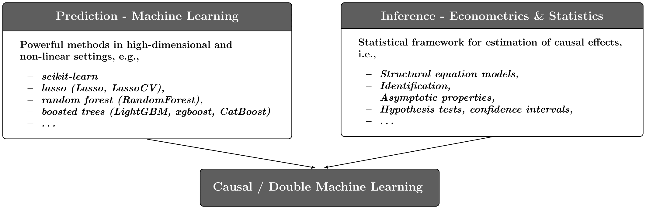
What is Double/Debiased Machine Learning (DML)?

• DML is a general framework for causal inference and estimation of causal parameters based on machine learning

• Summarized in Chernozhukov et al. (2018)

• Combines the strengths of machine learning and econometrics

What is Double/Debiased Machine Learning (DML)?

• Obtain a DML estimate of the causal parameter with asymptotically valid confidence intervals

• DML estimator has good theoretical statistical properties like \(\sqrt{N}\) rate of convergence, unbiasedness, approximate normality

• DML can be generalized to other causal models and settings (multiple treatments, heterogeneous treatment effects, \(\ldots\) )

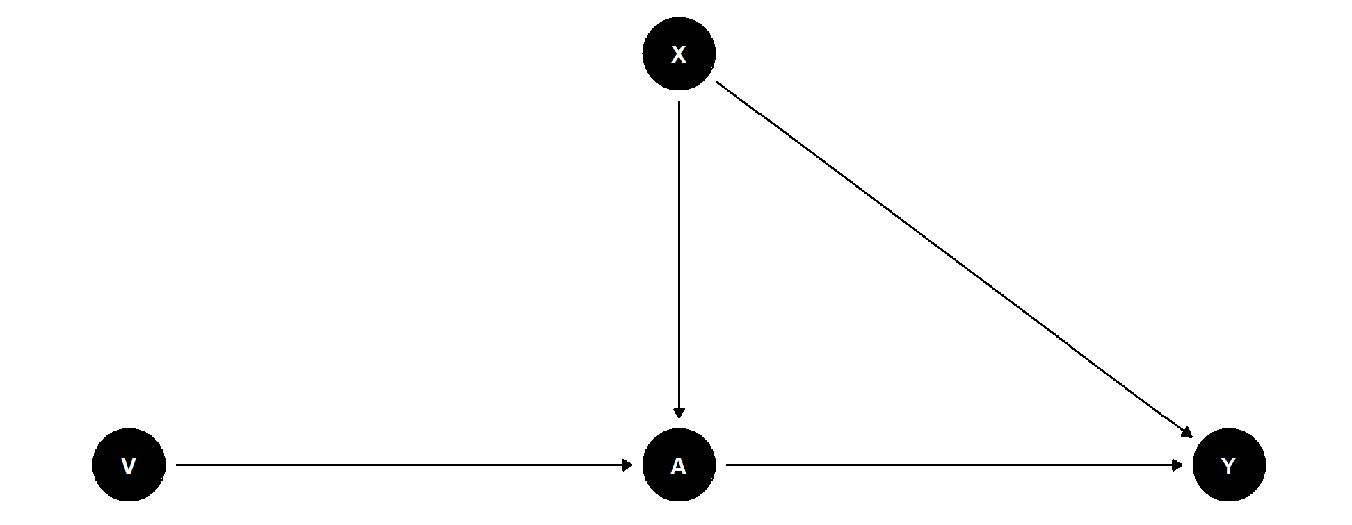
Motivating Example

Partially linear regression model (PLR)

\[\begin{align*} &Y = D \theta_0 + g_0(X) + \zeta, & &\mathbb{E}[\zeta | D,X] = 0, \\ &D = m_0(X) + V, & &\mathbb{E}[V | X] = 0, \end{align*}\]

with

• Outcome variable \(Y\)
• Policy or treatment variable of interest \(D\)
• High-dimensional vector of confounding covariates \(X = (X_1, \ldots, X_p)\)
• Stochastic errors \(\zeta\) and \(V\)

Introduction to Double Machine Learning

DML Key Ingredients

1. Neyman Orthogonality

• Inference is based on a moment condition that satisfies the Neyman orthogonality condition \(\psi(W; \theta, \eta)\) \[E[\psi(W; \theta_0, \eta_0)] = 0,\]

• where \(W:=(Y,D,X,Z)\) and with \(\theta_0\) being the unique solution that obeys the Neyman orthogonality condition \[\left.\partial_\eta \mathbb{E}[\psi(W; \theta_0, \eta] \right|_{\eta=\eta_0} = 0.\]

• \(\partial_{\eta}\) denotes the pathwise (Gateaux) derivative operator

DML Key Ingredients

1. Neyman Orthogonality

• Neyman orthogonality ensures that the moment condition identifying \(\theta_0\) is insensitive to small pertubations of the nuisance function \(\eta\) around \(\eta_0\)

• Using a Neyman-orthogonal score eliminates the first order biases arising from the replacement of \(\eta_0\) with a ML estimator \(\hat{\eta}_0\)

• PLR example: Partialling-out score function (cf. Section 5.3 , Appendix) \[\psi(\cdot)= (Y-E[Y|X]-\theta (D - E[D|X]))(D-E[D|X])\]

DML Key Ingredients

2. High-Quality Machine Learning Estimators

• The nuisance parameters are estimated with high-quality (fast-enough converging) machine learning methods.

• Different structural assumptions on \(\eta_0\) lead to the use of different machine-learning tools for estimating \(\eta_0\) Chernozhukov et al. (2018) (Section 3)

• Rate requirements depend on the causal model and orthogonal score, e.g. (see Chernozhukov et al. (2018)),

  • PLR, partialling out: \(\lVert \hat{m}_0 - m_0 \rVert_{P,2} \times \big( \lVert \hat{m}_0 - m_0 \rVert_{P,2} + \lVert \hat{\ell}_0 - \ell_0\rVert _{P,2}\big) \le \delta_N N^{-1/2}\)
  • IRM/DR score, ATE: \(\lVert \hat{m}_0 - m_0 \rVert_{P,2} \times \lVert \hat{\ell}_0 - \ell_0\rVert _{P,2} \le \delta_N N^{-1/2}\)

DML Key Ingredients

3. Sample Splitting

• To avoid the biases arising from overfitting, a form of sample splitting is used at the stage of producing the estimator of the main parameter \(\theta_0\).

• Efficiency gains by using cross-fittng (swapping roles of samples for train / hold-out)

DML Key Ingredients

Main result in Chernozhukov et al. (2018)

There exist regularity conditions, such that the DML estimator \(\tilde{\theta}_0\) concentrates in a \(1/\sqrt{N}\)-neighborhood of \(\theta_0\) and the sampling error is approximately \[\sqrt{N}(\tilde{\theta}_0 - \theta_0) \sim N(0, \sigma^2),\] with \[\begin{align}\begin{aligned}\sigma^2 := J_0^{-2} \mathbb{E}(\psi^2(W; \theta_0, \eta_0)),\\J_0 = \mathbb{E}(\psi_a(W; \eta_0)).\end{aligned}\end{align}\]

• See example based on Chernozhukov et al. (2018)

Practical Aspects of Double Machine Learning

Practical Aspects of DML

Questions in Practice

1. Which learner should be used for estimation of the nuisance parameter \(\eta_0\)?

   • In PLR example (partialling out): \(\eta_0=(\ell_0, m_0)=\big(\mathbb{E}[Y|X], \mathbb{E}[D|X]\big)\)

2. How should the hyperparameters of the learners be tuned? Which sample (splitting) to use for tuning?

3. Can AutoML frameworks be used? How well do they perform in practice?

4. Which causal model should be used?

Practical Aspects of DML

Approach

• Use various simulation settings and semi-synthetic benchmarks to elaborate role of practical choices
  • Choice of learner and hyperparameters
  • Parameter tuning
  • Sample splitting
  • Choice of causal models
  • \(\ldots\)

Goal

• Derive some guidance for applications of DML

Results

• First-stage error
• Estimation quality (\(MSE(\hat{\theta}_0)\), \(\ldots\))
• Emp. coverage
• Computation time

Motivating Example: Lasso Penalty

• How do more/less accurate estimators for \(\eta_0\) affect the causal estimate, \(\hat{\theta}\)?

• Relationship of nuisance fit and estimation quality

• Simulated example

  • high-dimensional linear sparse model, based on Belloni, Chernozhukov, and Hansen (2014)
  • \(n = 100\) and \(p=200\)
  • continuous treatment variable \(D\)

• Lasso learner for \(\eta_0 = (\ell_0, m_0)\) evaluated over a grid of \(\lambda = (\lambda_{\ell}, \lambda_{m})\) values (l1-penalty)

Motivating Example: Lasso Penalty

Motivating Example: Lasso Penalty

Motivating Example: Lasso Penalty

Motivating Example: Lasso Penalty

Simulation Results

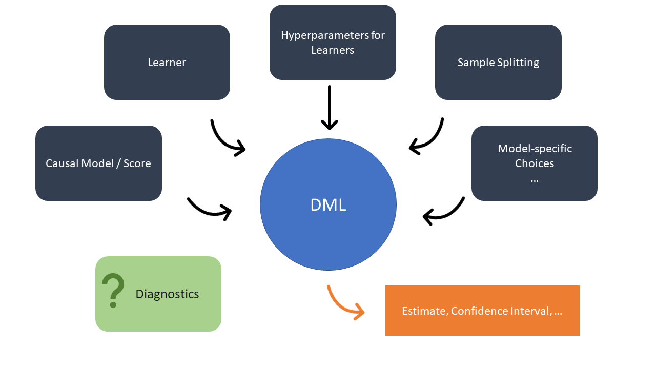
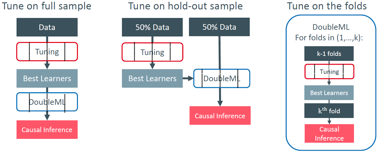
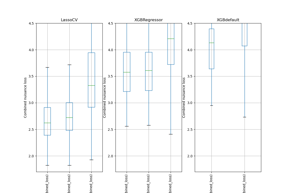
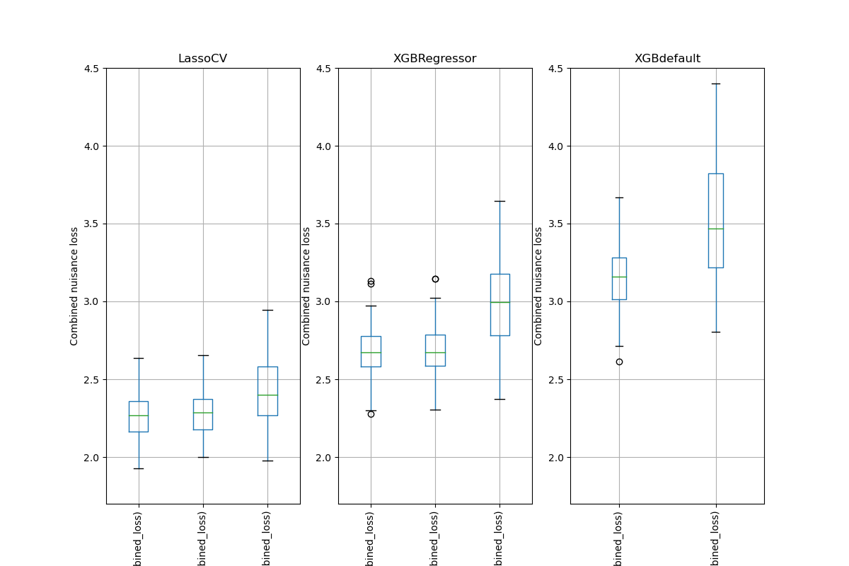
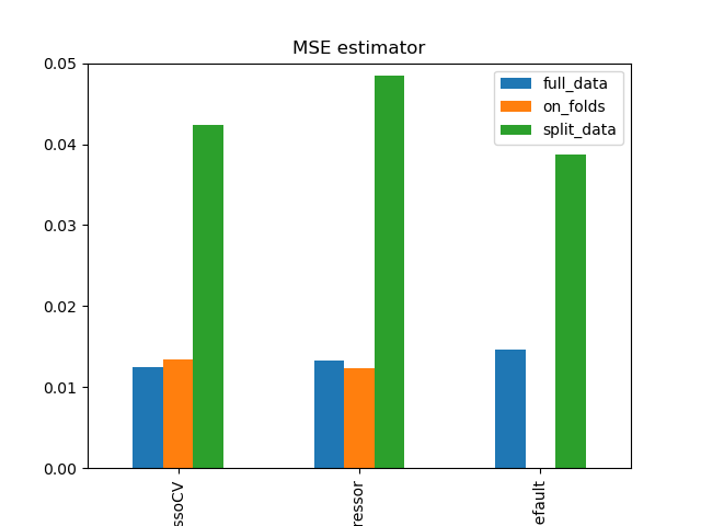
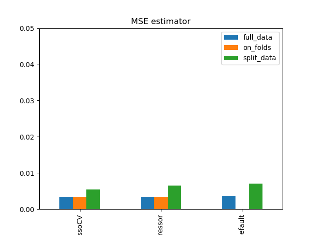
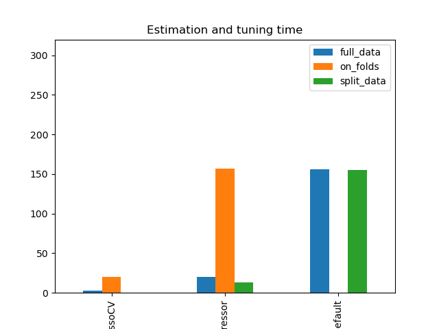
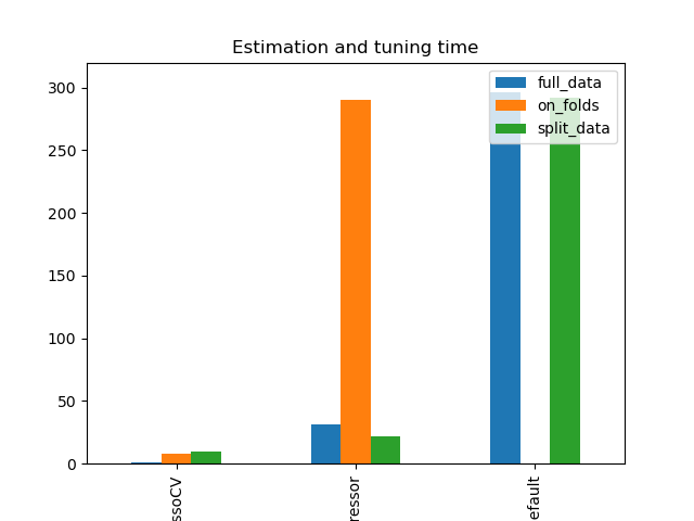
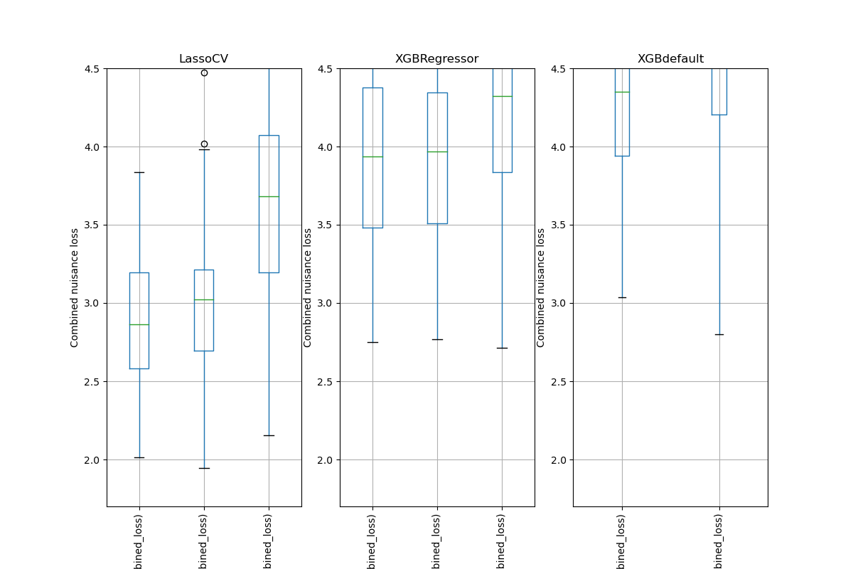
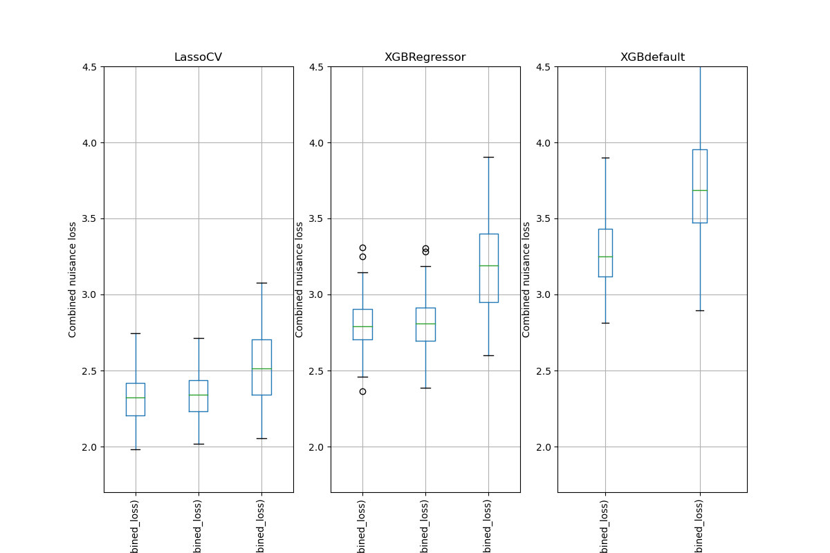
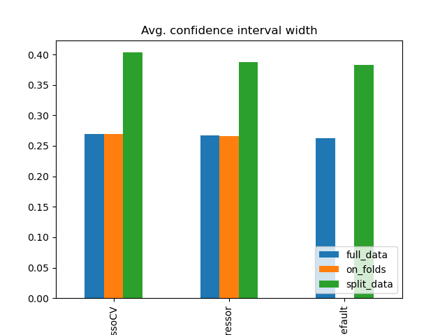
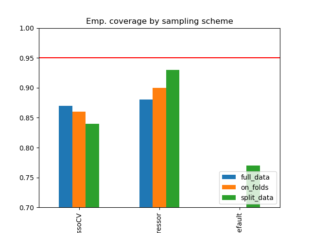
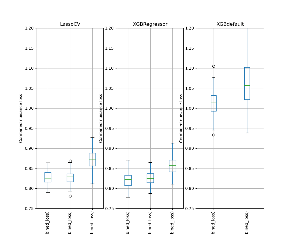
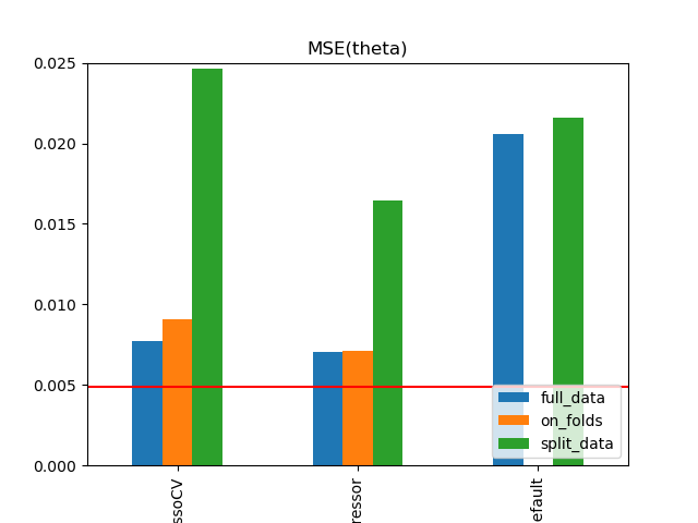
Sample Splitting and Hyperparameter Tuning

Canditate splitting schemes

Simulation Settings

Settings considered for PLR Model

• Setting 1: High-dimensional sparse and linear DGP as of Belloni, Chernozhukov, and Hansen (2014)
  • \(n = 100\), \(p = 200\)
  • \(n = 400\), \(p = 200\)
• Setting 2: “Scenario 2” from ACIC 2019 data challenge
  • PLR with nonlinear sparse specification for \(g_0(X)\) and \(m_0(X)\)
  • \(n=1000\), \(p=200\)
  • Binary treatment \(D\)

More settings

• ACIC2019 all DGPs
• IHDP Benchmark
• IRM model (AIPW/DR score)
• \(\ldots\)

Simulation Settings

Learners considered for PLR Model

• scikit-learn’s cross-validated Lasso (Pedregosa et al. 2011)
• XGBoost tuned (Chen et al. 2015)
• XGBoost default
• AutoML framework flaml (Wang et al. 2021)
• \(\ldots\)

Simulation Results: 1. BCH 2014

ml_l, n = 100

ml_l, n = 400

Figure 1: Nuisance fit, ml_l

Simulation Results: 1. BCH 2014

ml_m, n = 100

ml_m, n = 400

Figure 2: Nuisance fit, ml_m

Simulation Results: 1. BCH 2014

combined loss, n = 100

combined loss, n = 400

Figure 3: Nuisance fit, combined loss

Simulation Results: 1. BCH 2014

n = 100

n = 400

Figure 4: MSE(\(\hat{\theta}\))

Simulation Results: 1. BCH 2014

n = 100

n = 400

Figure 5: Empirical coverage

Simulation Results: 1. BCH 2014

n = 100

n = 400

Figure 6: CI width

Simulation Results: 1. BCH 2014

n = 100

n = 400

Figure 7: Estimation time

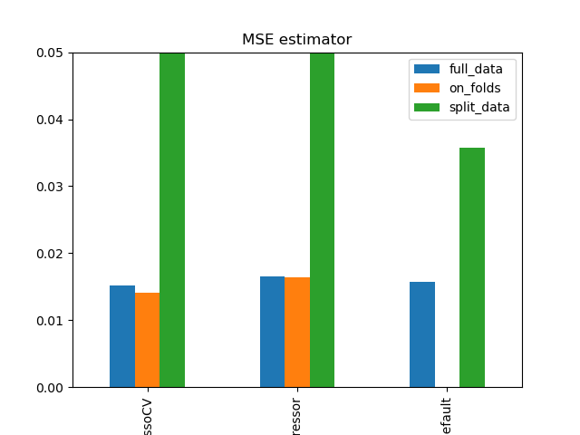
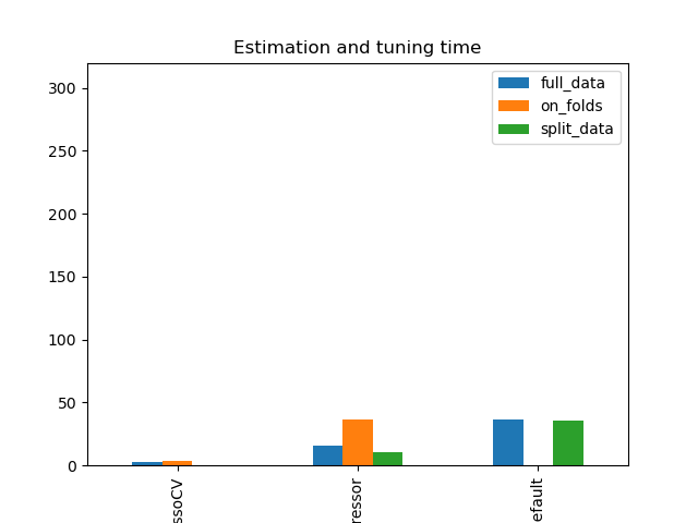
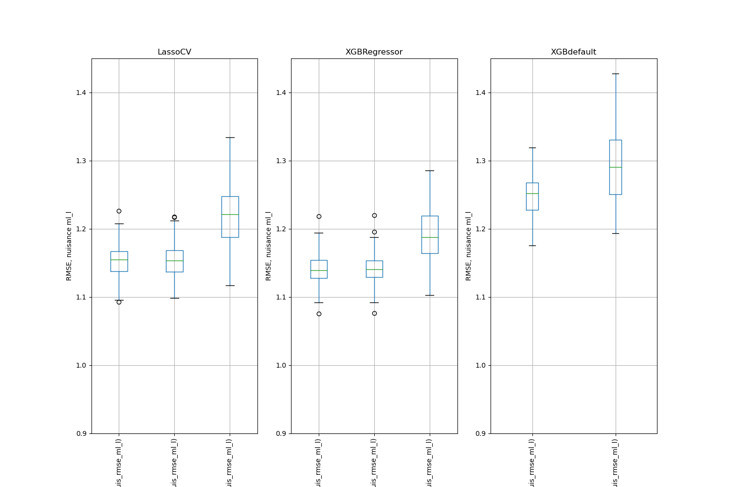
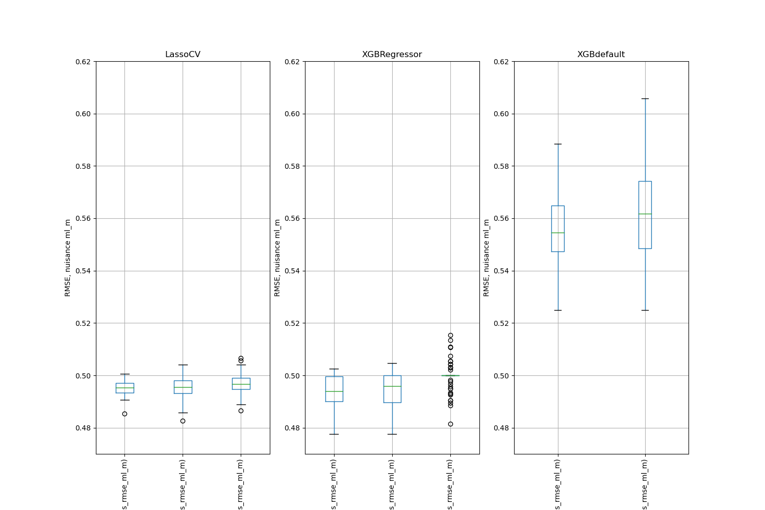
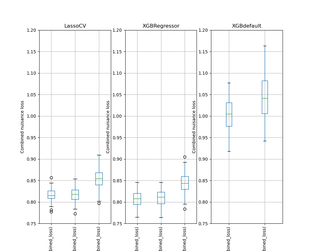
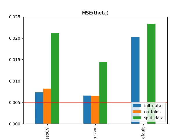
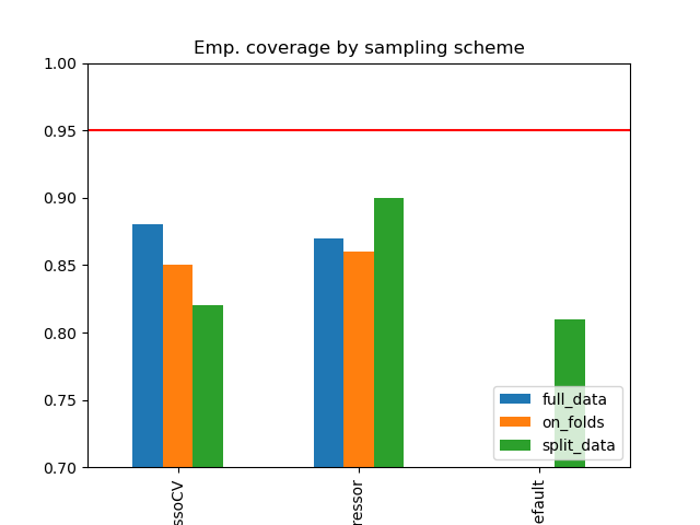
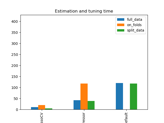
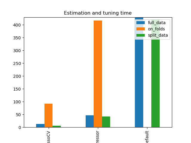
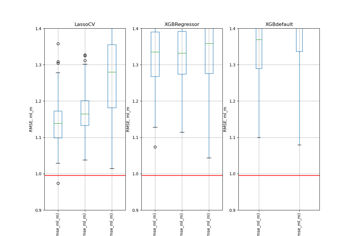
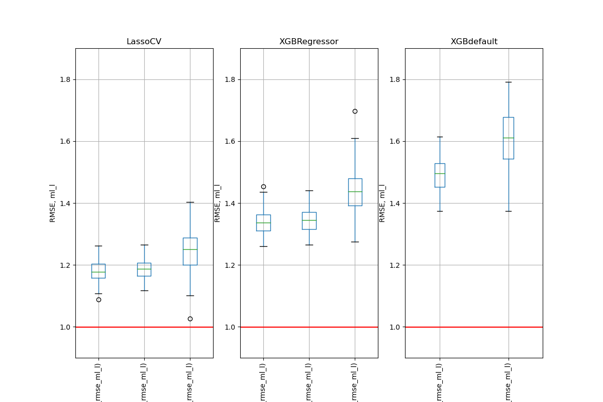
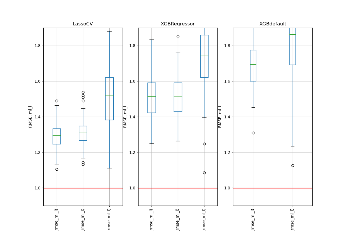
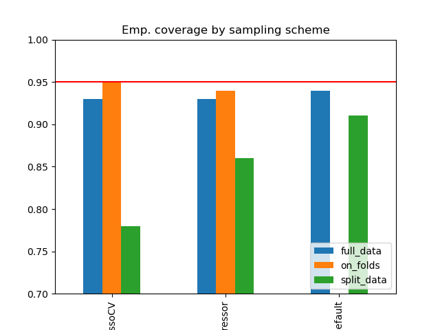
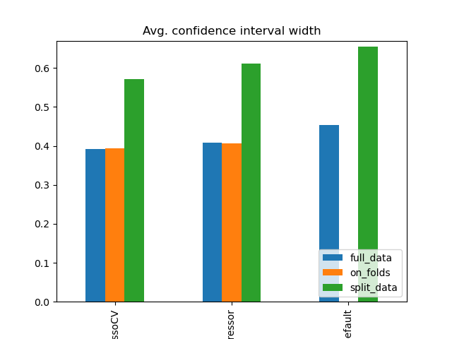
Simulation Results: 1. BCH 2014

Number of Folds for Cross-Fitting

n = 100, n_folds = 3

n = 100, n_folds = 10

Figure 8: Combined loss

Simulation Results: 1. BCH 2014

n = 400, n_folds = 3

n = 400, n_folds = 10

Figure 9: Combined loss

Simulation Results: 1. BCH 2014

n = 100, n_folds = 3

n = 100, n_folds = 10

Figure 10: MSE(\(\hat{\theta}\))

Simulation Results: 1. BCH 2014

n = 400, n_folds = 3

n = 400, n_folds = 10

Figure 11: MSE(\(\hat{\theta}\))

Simulation Results: 1. BCH 2014

n = 100, n_folds = 3

n = 100, n_folds = 10

Figure 12: Estimation time

Simulation Results: 1. BCH 2014

n = 400, n_folds = 3

n = 400, n_folds = 10

Figure 13: Estimation time

Simulation Results: 2. ACIC (DGP 2)

Nuisance fit, ml_l

Nuisance fit, ml_m

Figure 14: Nuisance fit

Simulation Results: 2. ACIC (DGP 2)

Combined loss

\(\text{MSE}(\hat{\theta}\))

Figure 15: Combined loss, MSE

Simulation Results: 2. ACIC (DGP 2)

CI width

Empirical coverage

Figure 16: CI width and emp. coverage

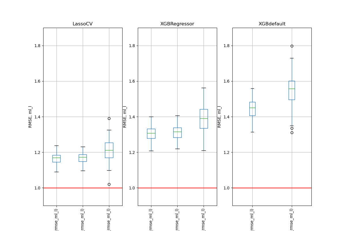
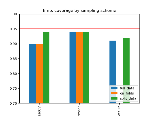
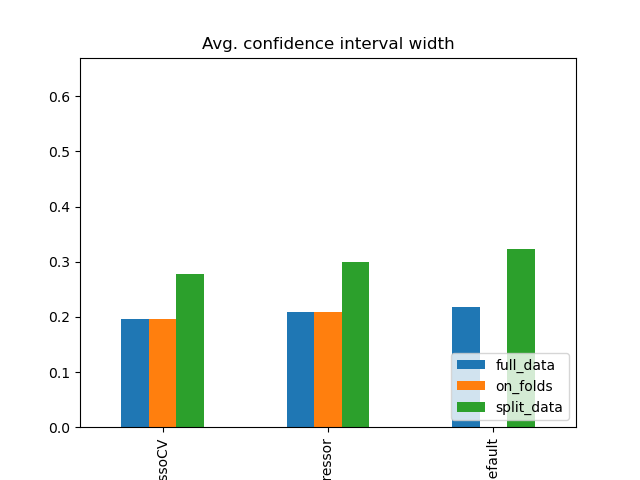
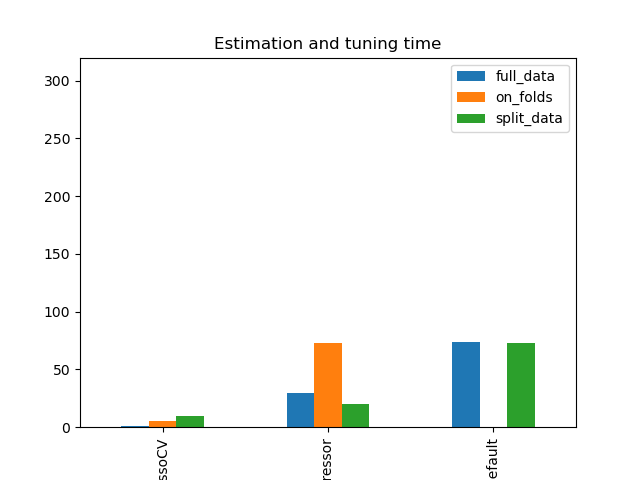
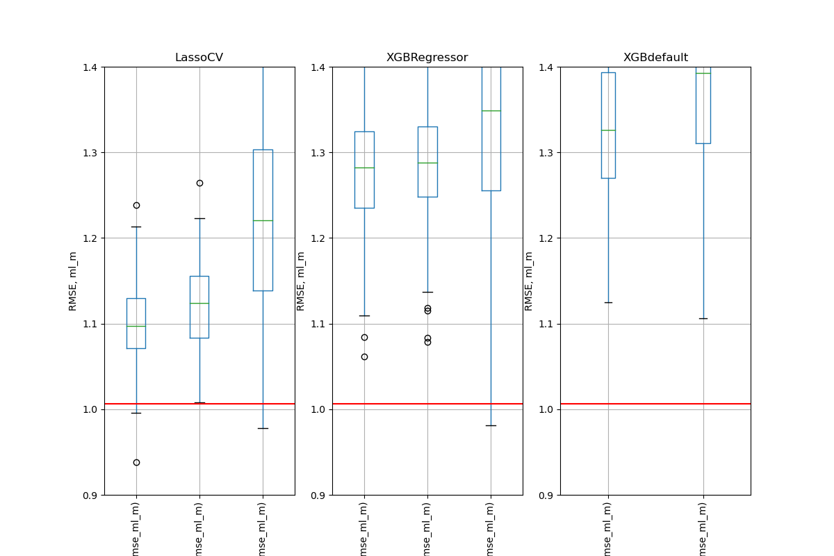
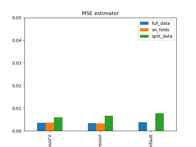
Simulation Results: 2. ACIC (DGP 2)

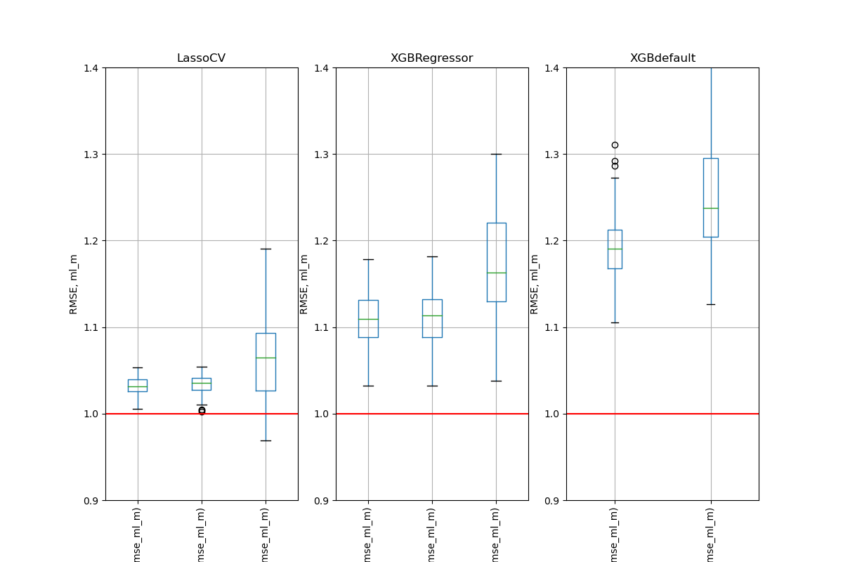
Number of Folds for Cross-Fitting

n_folds = 3

n_folds = 10

Figure 17: Combined loss

n_folds = 3

n_folds = 10

Figure 18: MSE

Simulation Results: 2. ACIC (DGP 2)

Empirical coverage, n_folds = 3

Empirical coverage, n_folds = 10

Figure 19: Emp. coverage

Simulation Results: 2. ACIC (DGP 2)

n_folds = 3

n_folds = 10

Figure 20: Estimation time

Simulation Results: 2. ACIC (DGP 2)

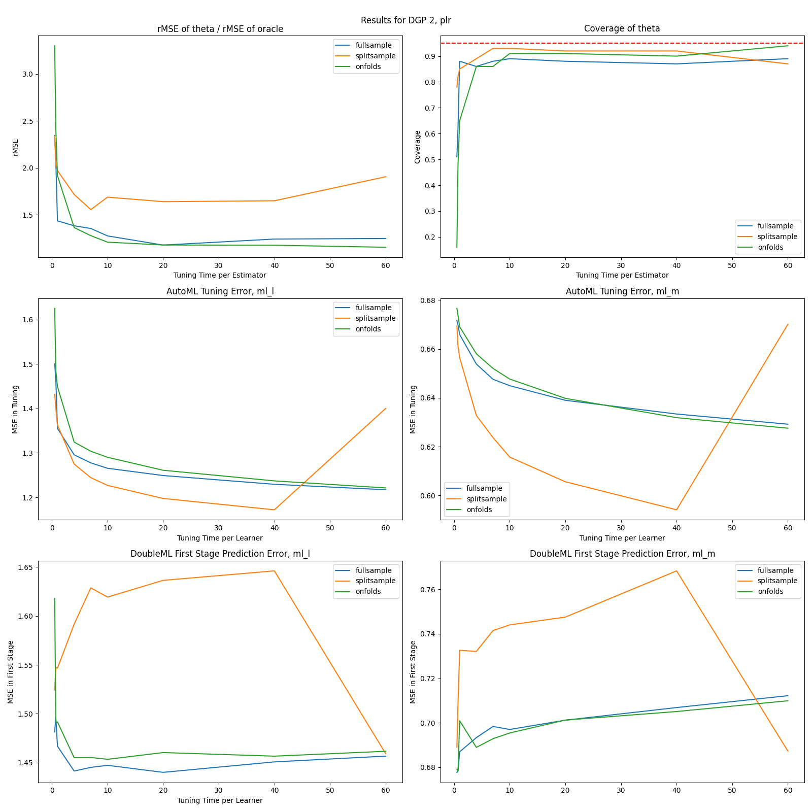
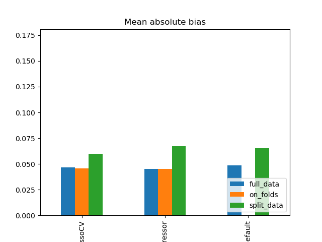
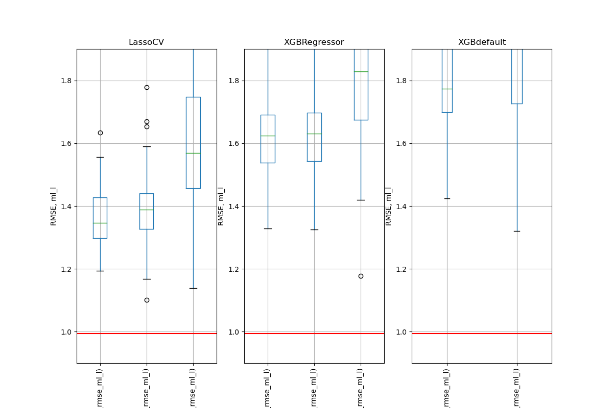
flaml, DGP 2

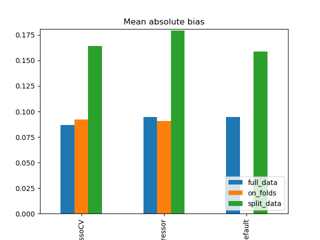
Simulation Results: 2. ACIC (all DGPs)

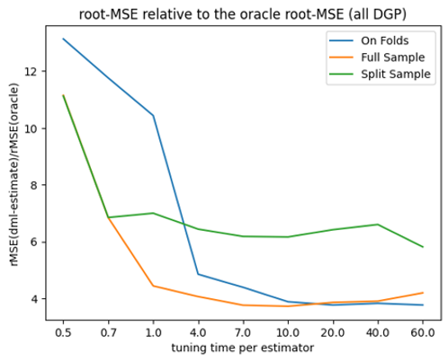
flaml, all DGPs

Summary

• Careful choice of learners and hyperparameter tuning is important for estimation quality for causal parameter \(\theta_0\)

• Full-sample and on-fold tuning seem to outperform the split-data approach in terms of

  • nuisance fit
  • estimation quality of \(\theta_0\)
  • coverage

• On-fold tuning computationally more expensive

• Lower (combined) first stage error found to be associated with better performance

Summary

• Higher number of folds for cross-fitting seem to improve the estimation performance, but at higher computational costs.
  • more important in small samples
  • can be evaluated empirically
• AutoML frameworks seem to work well in combination with DML
  • Some frameworks suffer from some instabilities

Next steps

• Choice of causal model / score

• Scale and summarize results, more benchmarks

• Evaluation of additional strategies:

  • Ensemble
  • Pick ‘best’ model
  • 1-se Lasso
  • \(\ldots\)

• Refined hyperparameter tuning

Appendix

DML Key Ingredients

1. Neyman Orthogonality

• The inference is based on a score function \(\psi(W; \theta, \eta)\) that satisfies \[E[\psi(W; \theta_0, \eta_0)] = 0,\]

• where \(W:=(Y,D,X,Z)\) and with \(\theta_0\) being the unique solution that obeys the Neyman orthogonality condition \[\left.\partial_\eta \mathbb{E}[\psi(W; \theta_0, \eta] \right|_{\eta=\eta_0} = 0.\]

• \(\partial_{\eta}\) denotes the pathwise (Gateaux) derivative operator

DML Key Ingredients

1. Neyman Orthogonality

• Neyman orthogonality ensures that the moment condition identifying \(\theta_0\) is insensitive to small pertubations of the nuisance function \(\eta\) around \(\eta_0\)

• Using a Neyman-orthogonal score eliminates the first order biases arising from the replacement of \(\eta_0\) with a ML estimator \(\hat{\eta}_0\)

• PLR example: Partialling-out score function (cf. Section 5.3 , Appendix) \[\psi(\cdot)= (Y-E[Y|X]-\theta (D - E[D|X]))(D-E[D|X])\]

Frisch-Waugh-Lovell Theorem

• Solution to regularization bias: Orthogonalization

• Remember the Frisch-Waugh-Lovell (FWL) Theorem in a linear regression model

\[Y = D \theta_0 + X'\beta + \varepsilon\]

• \(\theta_0\) can be consistently estimated by partialling out \(X\), i.e,

  1. OLS regression of \(Y\) on \(X\): \(\tilde{\beta} = (X'X)^{-1} X'Y\) \(\rightarrow\) Residuals \(\hat{\varepsilon}\)

  2. OLS regression of \(D\) on \(X\): \(\tilde{\gamma} = (X'X)^{-1} X'D\) \(\rightarrow\) Residuals \(\hat{\zeta}\)

  3. Final OLS regression of \(\hat{\varepsilon}\) on \(\hat{\zeta}\)

• Orthogonalization: The idea of the FWL Theorem can be generalized to using ML estimators instead of OLS

Neyman Orthogonality

Naive approach

\[\begin{align} \psi (W, \theta_0, \eta) = & (Y - D\theta_0 - g_0(X))D \end{align}\]

Regression adjustment score

\[\begin{align} \eta &= g(X), \\ \eta_0 &= g_0(X), \end{align}\]

FWL partialling out

\[\begin{align} \psi (W, \theta_0, \eta_0) = & ((Y- E[Y|X])-(D-E[D|X])\theta_0)\\ & (D-E[D|X]) \end{align}\]

Neyman-orthogonal score (Frisch-Waugh-Lovell)

\[\begin{align} \eta &= (g(X), m(X)), \\ \eta_0 &= ( g_0(X), m_0(X)) = ( \mathbb{E} [Y \mid X], \mathbb{E}[D \mid X]) \end{align}\]

Additional Results

Motivating Example: Lasso Penalty

Motivating Example: Lasso Penalty

Motivating Example: Lasso Penalty

Motivating Example: Lasso Penalty

Simulation Results: 1. BCH 2014

n = 100

n = 400

Figure 21: Absolute bias

Number of Folds for Cross-Fitting

Simulation Results: 1. BCH 2014

n = 100, n_folds = 3

n = 100, n_folds = 10

Figure 22: RMSE, ml_l

Simulation Results: 1. BCH 2014

n = 100, n_folds = 3

n = 100, n_folds = 10

Figure 23: RMSE, ml_m

Simulation Results: 1. BCH 2014

n = 400, n_folds = 3

n = 400, n_folds = 10

Figure 24: RMSE, ml_l

Simulation Results: 1. BCH 2014

n = 400, n_folds = 3

n = 400, n_folds = 10

Figure 25: RMSE, ml_m

Simulation Results: 2. ACIC (DGP 2)

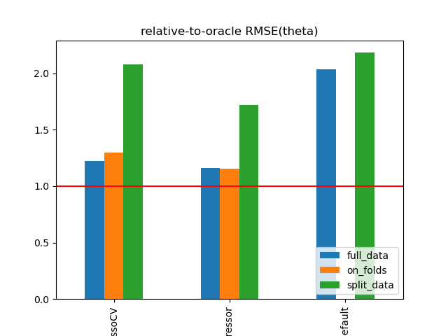
\(\text{rel. MSE}(\hat{\theta}\))

Simulation Results: 2. ACIC (DGP 2)

Abs. bias

IHDP Benchmark

TODO

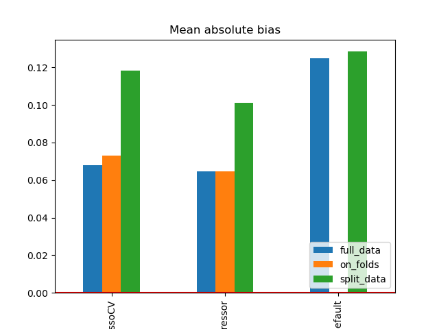
Resources

More resources

• For a nontechnical introduction to DML: Bach et al. (2021)

• Software implementation:

  • https://github.com/DoubleML/doubleml-for-py
  • https://github.com/DoubleML/doubleml-for-r
  • Docu and examples: docs.doubleml.org

• Paper draft to be uploaded at arxiv soon

::::

References

References

Bach, P., V. Chernozhukov, M. S. Kurz, and M. Spindler. 2021. “DoubleML – An Object-Oriented Implementation of Double Machine Learning in R.” https://arxiv.org/abs/2103.09603.

Belloni, Alexandre, Victor Chernozhukov, and Christian Hansen. 2014. “Inference on Treatment Effects After Selection Among High-Dimensional Controls.” The Review of Economic Studies 81 (2): 608–50.

Chen, Tianqi, Tong He, Michael Benesty, Vadim Khotilovich, Yuan Tang, Hyunsu Cho, Kailong Chen, et al. 2015. “Xgboost: Extreme Gradient Boosting.” R Package Version 0.4-2 1 (4): 1–4.

Chernozhukov, Victor, Denis Chetverikov, Mert Demirer, Esther Duflo, Christian Hansen, Whitney Newey, and James Robins. 2018. “Double/Debiased Machine Learning for Treatment and Structural Parameters.” The Econometrics Journal 21 (1): C1–68. https://onlinelibrary.wiley.com/doi/abs/10.1111/ectj.12097.

Pedregosa, Fabian, Gaël Varoquaux, Alexandre Gramfort, Vincent Michel, Bertrand Thirion, Olivier Grisel, Mathieu Blondel, et al. 2011. “Scikit-Learn: Machine Learning in Python.” Journal of Machine Learning Research 12 (85): 2825–30. http://jmlr.org/papers/v12/pedregosa11a.html.

Wang, Chi, Qingyun Wu, Markus Weimer, and Erkang Zhu. 2021. “FLAML: A Fast and Lightweight Automl Library.” Proceedings of Machine Learning and Systems 3: 434–47.