Double Machine Learning

Practical Considerations and Evidence from Extensive Simulation Experiments
Brown Bag Seminar, DICE, Düsseldorf
January 10, 2024

Philipp Bach, Sven Klaassen, Oliver Schacht, Martin Spindler

University of Hamburg and Economic AI

Agenda

• 1 Motivation
• 2 Introduction: Causal ML and DoubleML
• 3 Practical Aspects of Double Machine Learning
• 4 Appendix
• 5 References

1 Motivation

Motivation

• Causal Machine Learning (Causal ML) becomes increasingly popular in applied research

• Idea: Exploit the excellent predictive performance of ML methods for “better” estimation of causal effects

• Examples:

  • Regression models with high-dimensional control variables \(X\) (\(p>n\))
  • Nonlinear relationship between treatment \(D\), covariates \(X\) and outcome \(Y\)
  • Unstructured data (text and image data)

• Challenges
  • Use of predictive ML methods for causal inference is not straightforward
  • Open questions regarding practical choices in valid causal ML approaches (Chernozhukov et al. 2018)

This talk

Focus

Double/Debiased Machine Learning (DoubleML) (Chernozhukov et al. 2018)

DoubleML

• Valid estimation of a causal parameter (\(\theta_0\)) based on machine learning

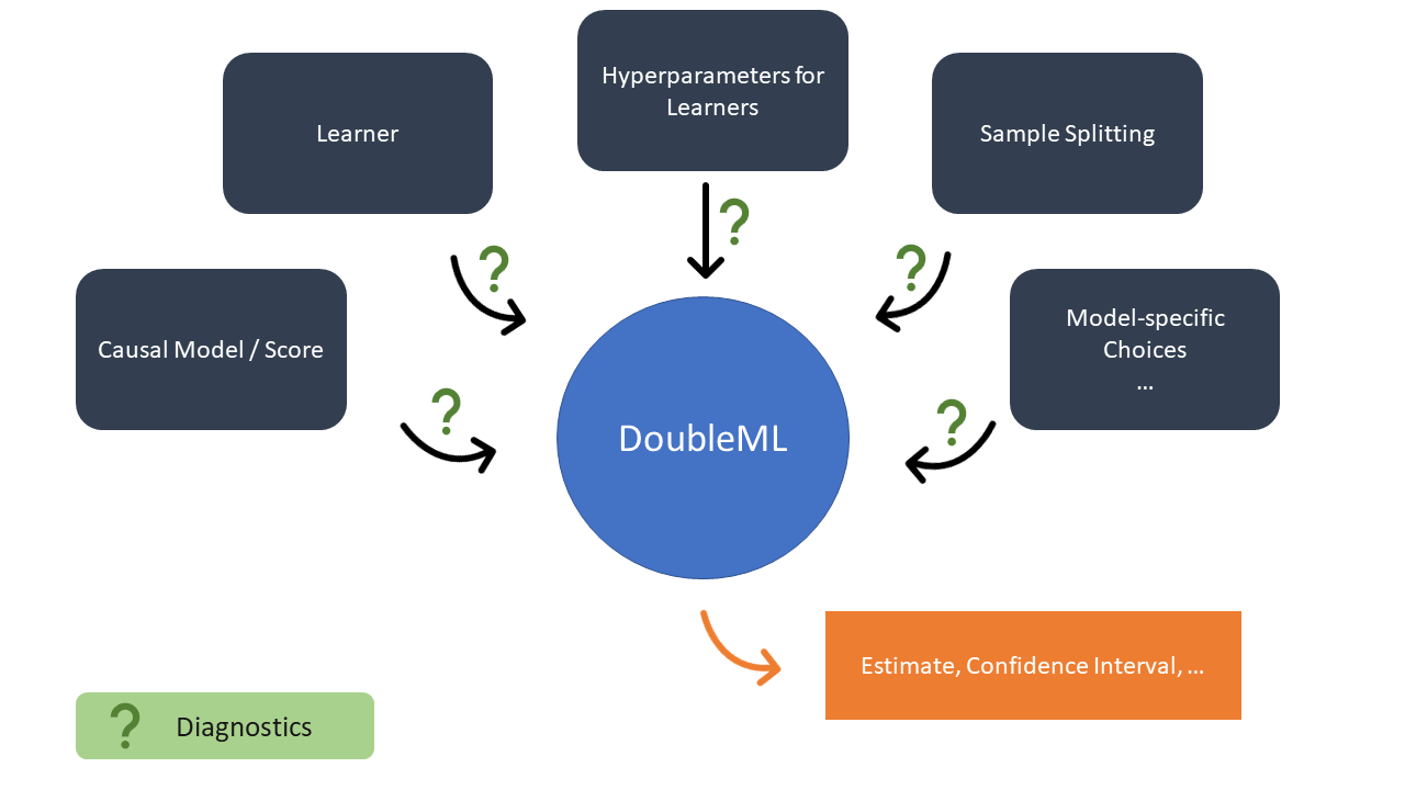
• 3 key ingredients: Orthogonality, ML Learner, Sample Splitting

• Open questions in practice

➡️ Evidence and recommendations based on extensive simulations

2 Introduction: Causal ML and DoubleML

What is DoubleML?

• DoubleML is a general framework for causal inference and estimation of causal parameters based on machine learning

• Summarized in Chernozhukov et al. (2018)

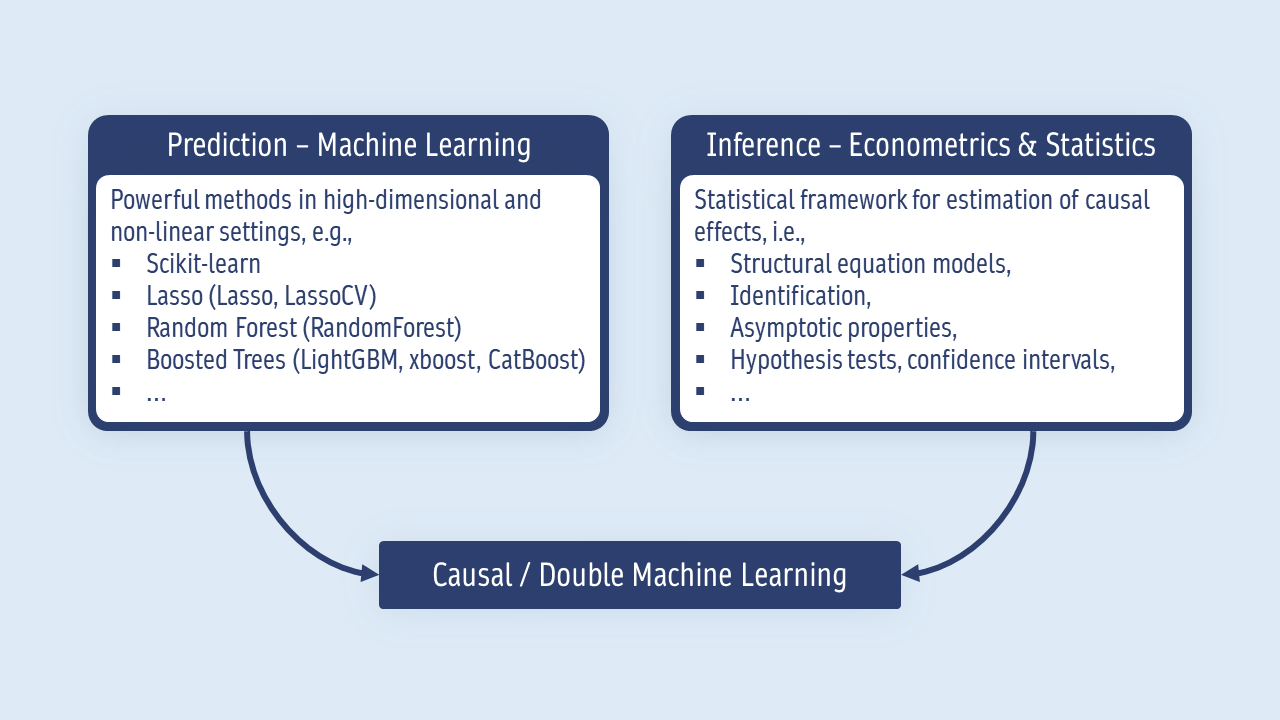
• Combines the strengths of machine learning and econometrics

What is DoubleML?

• Obtain a DoubleML estimate of a causal parameter with asymptotically valid confidence intervals in many different causal models

• DoubleML estimator has good theoretical statistical properties like \(\sqrt{N}\) rate of convergence, unbiasedness, approximate normality

• DoubleML Key Ingredients

  • Neyman orthogonality
  • High-quality ML learners
  • Sample splittings

• Various extensions of DoubleML available (e.g., multiple testing, heterogeneous treatment effects, diff-in-diff, sensitivity analysis)

Motivating Example

Partially linear regression model (PLR)

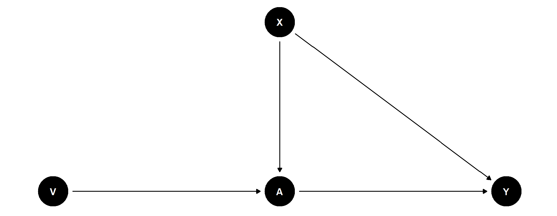
\[\begin{align*} &Y = D \theta_0 + g_0(X) + \zeta, & &\mathbb{E}[\zeta | D,X] = 0, \\ &D = m_0(X) + V, & &\mathbb{E}[V | X] = 0, \end{align*}\]

with

• Outcome variable \(Y\)
• Policy or treatment variable of interest \(D\)
• High-dimensional vector of confounding covariates \(X = (X_1, \ldots, X_p)\)
• Stochastic errors \(\zeta\) and \(V\)

DAG, conditional independence

Motivating Example

• Why can’t we simply plug in ML estimates \(\hat{g}_0(X)\) for \(g_0(X)\)?

\[\begin{align*} &Y = D \theta_0 + g_0(X) + \zeta, & &\mathbb{E}[\zeta | D,X] = 0. \end{align*}\]

⚡ Regularization bias

• Every ML method introduces some kind of regularization (implicitly or explicitly) to resolve the bias-variance tradeoff

• See this example based on Chernozhukov et al. (2018)

➡️ Adaption of the estimation framework necessary: Orthogonality

DoubleML Key Ingredients

1. Neyman Orthogonality

• In order to overcome the regularization bias, inference is based on a moment condition that satisfies the Neyman orthogonality condition

• Using a Neyman-orthogonal score eliminates the first order biases arising from the replacement of a so-called nuisance parameter \(\eta_0\) by an ML estimator \(\hat{\eta}_0\)

• PLR example: Partialling-out score function (cf. Frisch-Waugh-Lovell intuition in Section 4.2) \[\psi(\cdot)= (Y-E[Y|X]-\theta (D - E[D|X]))(D-E[D|X]),\]

• PLR nuisance parameter \(\eta_0 = (\ell_0(X), m_0(X)) = \big(\mathbb{E}[Y|X], \mathbb{E}[D|X] \big)\).

DoubleML Key Ingredients

2. High-Quality Machine Learning Estimators

• The nuisance parameters are estimated with high-quality (fast-enough converging) machine learning methods

• Chernozhukov et al. (2018): Different structural assumptions lead to the use of different machine-learning tools for estimating \(\eta_0\)

  • Example: Sparsity \(\rightarrow\) \(\ell_1\) penalized learners like lasso

• Formal requirements are specific to the causal model and orthogonal score
  • PLR, partialling out: \(\lVert \hat{m}_0 - m_0 \rVert_{P,2} \times \big( \lVert \hat{m}_0 - m_0 \rVert_{P,2} + \lVert \hat{\ell}_0 - \ell_0\rVert _{P,2}\big) \le \delta_N N^{-1/2}\)
  • IRM, doubly robust score, ATE: \(\lVert \hat{m}_0 - m_0 \rVert_{P,2} \times \lVert \hat{\ell}_0 - \ell_0\rVert _{P,2} \le \delta_N N^{-1/2}\)

DoubleML Key Ingredients

3. Sample Splitting

• To avoid the biases arising from overfitting, a form of sample splitting is used at the stage of producing the estimator of the main parameter \(\theta_0\).

• Efficiency gains by using cross-fitting (swapping roles of samples for train / hold-out)

Main result in Chernozhukov et al. (2018)

There exist regularity conditions, such that the DoubleML estimator \(\tilde{\theta}_0\) concentrates in a \(1/\sqrt{N}\)-neighborhood of \(\theta_0\) and the sampling error is approximately \[\sqrt{N}(\tilde{\theta}_0 - \theta_0) \sim N(0, \sigma^2),\] with \[\begin{align}\begin{aligned}\sigma^2 := J_0^{-2} \mathbb{E}(\psi^2(W; \theta_0, \eta_0)),\\J_0 = \mathbb{E}(\psi_a(W; \eta_0)).\end{aligned}\end{align}\]

• See example based on Chernozhukov et al. (2018)

3 Practical Aspects of Double Machine Learning

Frequently Asked Questions: DoubleML

1. How does the predictive performance of the ML learners translate into causal estimation quality?

2. How to choose learners? Can we use AutoML?

3. Do we need to tune hyperparameters for the learners? If so, how?

4. How to split the sample for tuning and for causal estimation (cross-fitting)?

5. Which causal model should be used?

❗ Simulation study

Simulation Study

Approach

• Use simulation settings and semi-synthetic benchmarks to elaborate role of practical choices

Goal

• Shed light on relationship of ML prediction and causal estimation

• Derive some guidance and diagnostics for applications of DoubleML

Settings

• Simulation settings
  • Atlantic Causal Inference Conference Data Challence 2019 (ACIC)
  • Belloni, Chernozhukov, and Hansen (2014)
• Semi-synthetic setting
  • IHDP benchmark

Nuisance Fit and Causal Estimation Quality

Relationship of nuisance fit and estimation quality

How do more or less accurate prediction for \(\eta_0\) affect the causal estimate, \(\hat{\theta}\)?

• High-dimensional linear sparse simulation setting based on Belloni, Chernozhukov, and Hansen (2014)

• Lasso learner for \(\eta_0 = (\ell_0, m_0)\) evaluated over a grid of \(\lambda = (\lambda_{\ell}, \lambda_{m})\) values (l1-penalty)

Motivating Example: Lasso Penalty

Motivating Example: Lasso Penalty

Motivating Example: Lasso Penalty

Motivating Example: Observations

• A proper choice of \(\lambda\) is crucial for good causal estimation (low \(MSE(\theta)\), high coverage)

• Low values for the combined loss correspond to lower MSE and higher empirical coverage

• We can also relate the empirical coverage to the first-stage prediction error for \(\eta_0 = (\ell_0, m_0)\), see Section 4.5

• Lower prediction errors are associated with lower \(MSE(\theta)\) and higher empirical coverage

• The results are obtained in a stylized high-dimensional sparse setting and are in line with the theory

➡️ Can we make similar observations in more realistic scenarios?

ACIC 2019

• ACIC 2019 data: Simulated data set for challenge that exhibit common patterns in economic data sets from external source

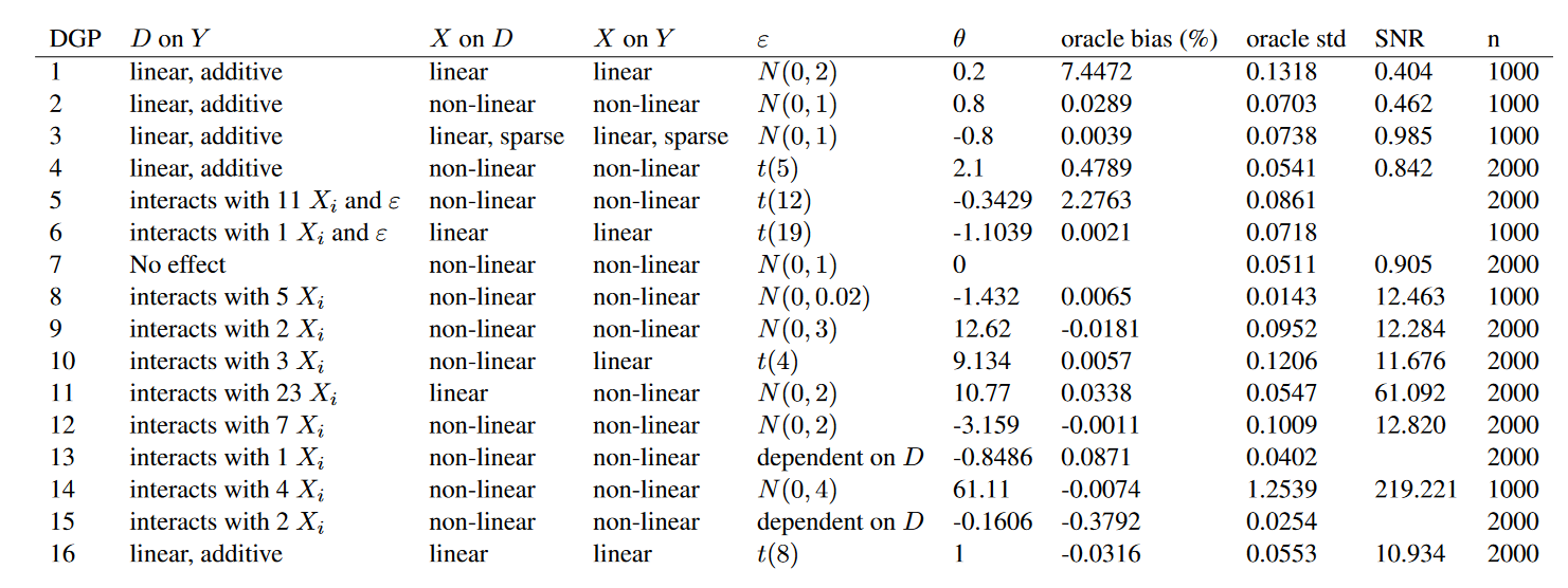
• 1600 data sets generated from 16 (very) different DGPs, mostly under conditional independence assumption. DGPs differ in terms of structural assumptions

  • Sparse vs. dense settings
  • Linear vs. nonlinear settings
  • Additively separable causal effect vs. interactions
  • Constant vs. heterogeneous tretment effect

• Binary treatment \(D\), continuous outcome \(Y\), \(p=200\) covariates, \(n\in \{1000, 2000\}\) observations, cf. Table in Section 4.11

ACIC 2019

• Causal parameter: Average treatment effect (ATE) \[ATE = \mathbb{E}[Y(1) - Y(0)]\]

• Causal models used:

  • PLR model: Constant treatment effect, additively separable, partially linear

  • Nonparametric model (“IRM”): Heterogeneous treatment effect, no functional form assumption

\[Y = D \theta_0 + g_0(X) + \zeta\]

\[Y = g_0(D, X) + U\]

• Challenge website: https://sites.google.com/view/acic2019datachallenge/data-challenge

ACIC 2019

In the ACIC 2019 data and real-data applications, we cannot rely on preliminary knowledge on the structural assumptions of the underlying model …

❓ Which learner should we pick and how?

❓ How should we choose the hyperparameters for these learners?

❓ How should we split the sample for parameter tuning and causal estimation?

❓ Which causal model should we use?

Learners and Hyperparameter Grids

Learners and Tuning Grids

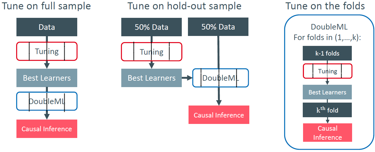
Sample Splitting and Hyperparameter Tuning

• Sample splitting is used for
  • Hyperparameter tuning (cross-validation)
  • Cross-fitting in DoubleML

Canditate splitting schemes

Results: Sample Splitting

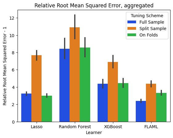
rRMSE (\(\hat{\theta}_0\)), ACIC 2019

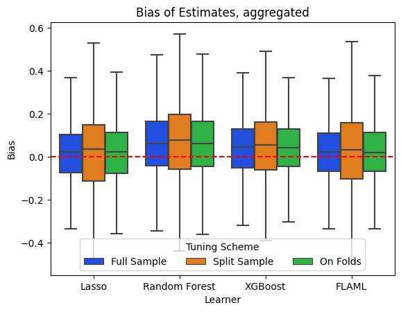
Bias (\(\hat{\theta}_0\)), ACIC 2019

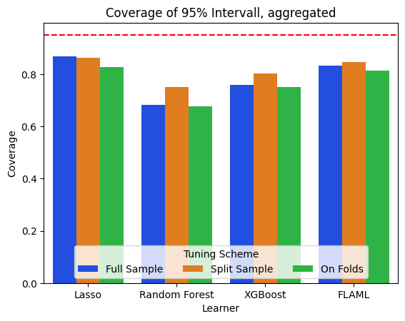
Empirical coverage, ACIC 2019

• Tuning on the full sample or on folds exhibit similar performance, which is superior to the split sample approach in small samples

Results: Sample Splitting

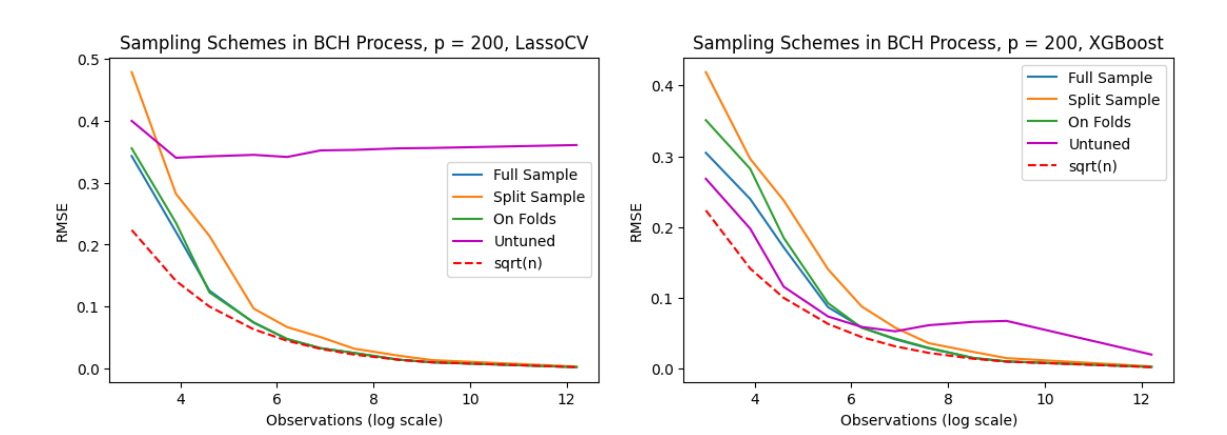
RMSE (\(\hat{\theta}_0\)), sample splitting, with increasing \(n\) (BCH)

• The efficiency loss of the split sample approach vanishes with increasing sample size.

Results: Learners

rRMSE, ACIC 2019

Bias, ACIC 2019

Empirical coverage, ACIC 2019

• The causal estimation quality depends on structural assumptions (sparsity, density) and appropriate learner choice

• Proper parameter tuning is crucial for good estimation performance

• In ACIC 2019, we find that AutoML and lasso perform best

Results: Selection of Learners

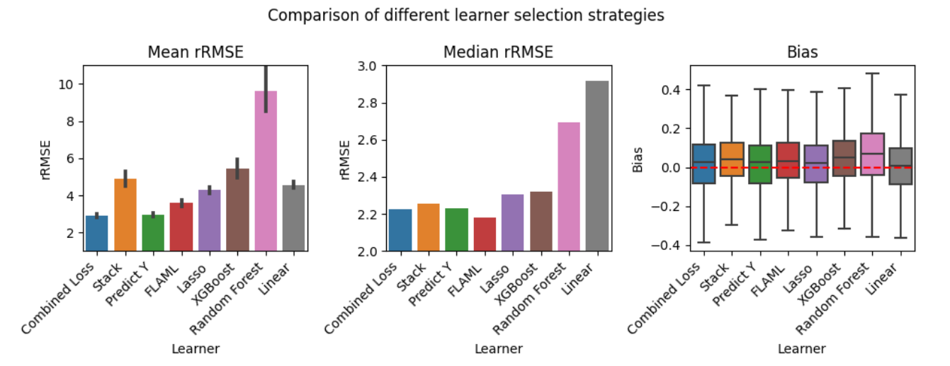
Learner selection strategies, full sample scheme, ACIC 2019

• A lower combined nuisance loss is associated with better causal estimation

• Low signal-to-noise ratios create challenges in small samples

• Combined nuisance loss serves as a good learner selection metric for causal estimation

Results: Choice of Causal Model

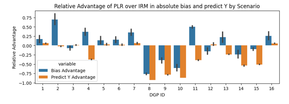
• The predictive performance of the causal models provides guidance on the choice of the causal model

• Efficiency gains can be achieved by exploiting a partially linear structure if partial linearity holds in the true model, more details in Section 4.13

Application: IHDP¹

Method	MAE ± std. err.
DML with FLAML	0.111 ± 0.009
RieszNet (Chernozhukov et al. 2022)	0.110 ± 0.003
Dragonnet (Shi, Blei, and Veitch 2019)	0.146 ± 0.010
CausalForest (Athey, Tibshirani, and Wager 2019)	0.728 ± 0.028

1. IHDP was a randomized control trial, studying the effect of certain measures (i.e. attendance at specialized clinics) of low birth weight infants on future developmental and health outcomes. We use \(1000\) generated datasets of 747 observations as in Chernozhukov et al. (2022). Each observation consists of an outcome \(Y\), a binary treatment \(T\) and \(25\) confounders \(X\) that can are continuous or binary.

Summary

• Good predictive performance by ML methods is associated with better causal estimation

• Careful choice of learners and hyperparameters is crucial for good causal estimation quality

• AutoML frameworks seem to work well in combination with DoubleML (adaptivity to different settings)

• Combined first stage error seems to serve as a good learner selection rule

Summary

• Full-sample and on-fold tuning seem to outperform the split-data approach in small samples in terms of nuisance fit, estimation quality of \(\theta_0\), empirical coverage

• The efficiency loss for split sample approach vanishes in bigger samples

• The predictive performance of the causal models can be exploited to motivate a specific model choice

Recommendations

General recommendations

• Address the predictive performance of the ML methods transparently and critically

• Provide context, insights and diagnostics to the robustness of the causal estimates

• Include benchmarks such as linear or logistic regression

Recommended diagnostics

• First-stage error (e.g., RMSE)

• Combined loss (specific to causal model and score)

• Range for causal estimates according to different learners / parameters

• Evaluate predictive performance of the causal models

Thank you

Thank you for your attention!

Slides and working paper available at

https://philippbach.github.io/notebooks.html

Additional Resources

• For a nontechnical introduction to DoubleML: Bach, Chernozhukov, Klaassen, et al. (2021)

• Software implementation:

  • https://github.com/DoubleML/doubleml-for-py
  • https://github.com/DoubleML/doubleml-for-r
  • Extensive docu and examples: docs.doubleml.org

4 Appendix

DoubleML Key Ingredients

1. Neyman Orthogonality

• In order to overcome the regularization bias, inference is based on a moment condition that satisfies the Neyman orthogonality condition \[E[\psi(W; \theta_0, \eta_0)] = 0,\]

• where \(\psi(W; \theta, \eta)\) is a score function, \(W\) denotes the data and \(\theta_0\) is the unique solution that obeys the Neyman orthogonality condition \[\left.\partial_\eta \mathbb{E}[\psi(W; \theta_0, \eta)] \right|_{\eta=\eta_0} = 0.\]

• \(\partial_{\eta}\) denotes the pathwise (Gateaux) derivative operator

• Neyman orthogonality ensures that the moment condition identifying \(\theta_0\) is insensitive to small pertubations of the nuisance function \(\eta\) around \(\eta_0\)

Frisch-Waugh-Lovell Theorem

• Solution to regularization bias: Orthogonalization

• Remember the Frisch-Waugh-Lovell (FWL) Theorem in a linear regression model

\[Y = D \theta_0 + X'\beta + \varepsilon\]

• \(\theta_0\) can be consistently estimated by partialling out \(X\), i.e,

  1. OLS regression of \(Y\) on \(X\): \(\tilde{\beta} = (X'X)^{-1} X'Y\) \(\rightarrow\) Residuals \(\hat{\varepsilon}\)

  2. OLS regression of \(D\) on \(X\): \(\tilde{\gamma} = (X'X)^{-1} X'D\) \(\rightarrow\) Residuals \(\hat{\zeta}\)

  3. Final OLS regression of \(\hat{\varepsilon}\) on \(\hat{\zeta}\)

• Orthogonalization: The idea of the FWL Theorem can be generalized to using ML estimators instead of OLS

Neyman Orthogonality

The naive plug-in approach minimizes the following MSE

\[\begin{align} min_{\theta} \mathbb{E}[(Y - D\theta_0 - g_0(X))^2] \end{align}\]

This implies the following moment equation

\[\begin{align} \mathbb{E}[\underbrace{(Y - D\theta_0 - g_0(X))D}_{=:\psi (W, \theta_0, \eta)}]&=0 \end{align}\]

Whereas for the partialling-out approach minimizes

\[\begin{align} min_{\theta} \mathbb{E}\big[\big(Y - \mathbb{E}[Y|X] - (D-\mathbb{E}[D|X])\theta\big)^2\big] \end{align}\]

which implies

\[\begin{align} \mathbb{E}\big[\underbrace{\big(Y - \mathbb{E}[Y|X] - (D-\mathbb{E}[D|X])\theta\big)(D-\mathbb{E}[D|X])}_{=:\psi (W, \theta_0, \eta)}\big]&=0 \end{align}\]

Neyman Orthogonality

Naive approach

\[\begin{align} \psi (W, \theta_0, \eta) = & (Y - D\theta_0 - g_0(X))D \end{align}\]

Regression adjustment score

\[\begin{align} \eta &= g(X), \\ \eta_0 &= g_0(X), \end{align}\]

FWL partialling out

\[\begin{align} \psi (W, \theta_0, \eta_0) = & ((Y- E[Y|X])-(D-E[D|X])\theta_0)\\ & (D-E[D|X]) \end{align}\]

Neyman-orthogonal score (Frisch-Waugh-Lovell)

\[\begin{align} \eta &= (g(X), m(X)), \\ \eta_0 &= ( g_0(X), m_0(X)) = ( \mathbb{E} [Y \mid X], \mathbb{E}[D \mid X]) \end{align}\]

Motivating Example: Lasso Penalty

Motivating Example: Lasso Penalty

Motivating Example: Lasso Penalty

Motivating Example: Lasso Penalty

Motivating Example: Lasso Penalty

Motivating Example: Lasso Penalty

DGPs: ACIC 2019

DGPs, ACIC 2019

Metrics, ACIC 2019

Metrics, ACIC 2019

Additional Results: Selection of Learners

Combined loss vs. bias (\(\theta\)), increasing \(n\) (BCH)

Additional Results: Choice of Causal Model

• The predictive performance of the causal models provides guidance on the choice of the causal model

Additional Results: Choice of Causal Model

Additional Results: Relation to ACIC Challenge

Relation to ACIC challenge results

5 References

References

Athey, Susan, Julie Tibshirani, and Stefan Wager. 2019. “Generalized Random Forests.”

Bach, Philipp, Victor Chernozhukov, Sven Klaassen, Malte S Kurz, and Martin Spindler. 2021. “DoubleML – An Object-Oriented Implementation of Double Machine Learning in R.” https://arxiv.org/abs/2103.09603.

Bach, Philipp, Victor Chernozhukov, Malte S Kurz, and Martin Spindler. 2021. “DoubleML – An Object-Oriented Implementation of Double Machine Learning in Python.” arXiv Preprint arXiv:2104.03220.

Belloni, Alexandre, Victor Chernozhukov, and Christian Hansen. 2014. “Inference on Treatment Effects After Selection Among High-Dimensional Controls.” The Review of Economic Studies 81 (2): 608–50.

Chernozhukov, Victor, Denis Chetverikov, Mert Demirer, Esther Duflo, Christian Hansen, Whitney Newey, and James Robins. 2018. “Double/Debiased Machine Learning for Treatment and Structural Parameters.” The Econometrics Journal 21 (1): C1–68. https://onlinelibrary.wiley.com/doi/abs/10.1111/ectj.12097.

Chernozhukov, Victor, Whitney K. Newey, Victor Quintas-Martinez, and Vasilis Syrgkanis. 2022. “RieszNet and ForestRiesz: Automatic Debiased Machine Learning with Neural Nets and Random Forests.” https://arxiv.org/abs/2110.03031.

Shi, Claudia, David M. Blei, and Victor Veitch. 2019. “Adapting Neural Networks for the Estimation of Treatment Effects.” https://arxiv.org/abs/1906.02120.