Causal Machine Learning and Sensitivity Analysis for Difference-in-Differences Models

Philipp Bach, Sven Klaassen, Jannis Kück, Mara Mattes, Martin Spindler

May 22, 2024

Outline

Double Machine Learning for Difference-in-Difference Models

Sensitivity Analysis for DoubleML

Sensitivity Analysis for Difference-in-Difference Models

Challenges and Outlook

Double Machine Learning for Difference-in-Difference Models

DoubleML for DiD

Difference-in-Differences (DiD) is “the single most popular research design in the quantitative social sciences”

Cunningham (2021, chap. 9)

Recent Developments

1️⃣ Difference-in-Differences

2️⃣ Causal Machine Learning

3️⃣ Sensitivity Analysis

DoubleML, DiD, Sensitivity: Recent developments

1️⃣ Difference-in-Differences

• TWFE limitations, multiple treatment periods, staggered treatment adoption, \(\ldots\)
• Literature: Roth et al. (2023), De Chaisemartin and d’Haultfoeuille (2023), Callaway (2023) (\(\ldots\))

2️⃣ Causal Machine Learning

• Double Machine Learning (DML) (Chernozhukov et al. 2018)
• DML for DiD: Chang (2020), Zimmert (2018), Sant’Anna and Zhao (2020)

3️⃣ Sensitivity Analysis

• Formal sensitivity analysis (linear regression) (Cinelli and Hazlett 2020)
• Generalization to debiased ML (Chernozhukov et al. 2022)

DoubleML, DiD, Sensitivity: Recent developments

Outlook: This Project

• Difference-in-Difference models depend crucially on the assumption of (conditional) parallel trends (PT)

• However, how robust are DiD study results to violations of PT?

  • Time-varying confounding
  • Unobserved pre-treatment confounders
  • Functional form misspecification
  • Anticipation
  • Spillovers

• Idea: Develop framework for sensitivity analysis w.r.t. violations of PT

• Related literature: Chernozhukov et al. (2022), Rambachan and Roth (2023)

DML for DiD

Introduction to DML (Chernozhukov et al. 2018)

• Estimation framework for causal parameter(s) \(\theta_0\) based on ML estimation

• General challenge of Causal ML:

  • ML algorithms introduce regularization bias (bias variance trade-off)
  • Regularization bias can lead to inconsistent estimation of causal parameters
  • ⚠️ Invalid inference (biased estimate, non-normal asymptotics)

Key ingredients of DML

1. Neyman Orthogonality
2. High-quality machine learning estimators
3. Sample splitting

DML for DiD

Introduction to DML (Chernozhukov et al. 2018)

• DML is an estimation framework based on a causal model and corresponding identification assumptions
  • Example: ATET in DiD and its group aggregations under (conditional) parallel trends, no anticipation and common support

• DML is a method-of-moments estimator, i.e.,
  • The underlying moment condition satisfies the property of Neyman Orthogonality
  • The moment condition is specific to a causal model and the parameter of interest and usually available from the literature (e.g., doubly robust for DiD)
• In words: The moment condition that is used to identify \(\theta_0\) is insensitive to small biases arising from regularization, i.e., immunized against first-order biases from regularization

Additional example and technical details available in Appendix 1.

DML for DiD

Introduction to DML (Chernozhukov et al. 2018)

• DML gives rise to a consistent and asymptotically normally distributed estimator of \(\theta_0\) that is robust to regularization bias

• DML applies to a wide range of causal models in empirical economic research

• Compatible with basically all ML methods (as long as they satisfy a quality criterion)

• Sample splitting is required to abstract from overfitting biases which would affect the effect estimation

DML for DiD: Setting

Setting: 2 Time Periods

• Two time periods:

  • \(t=0\) pre-treatment
  • \(t=1\) post-treatment

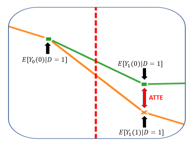
• \(Y_{t}\): Outcome of interest at time \(t\)

• \(D_{}\): Treatment indicator if treated between \(t=0\) and \(t=1\) (binary treatment)

• \(Y_{t}(0)\): Potential outcome of interest at time \(t\) if not treated up until \(t\)

• \(Y_{t}(1)\): Potential outcome of interest at time \(t\) if treated up until \(t\)

Motivation

Key assumption: Parallel trends

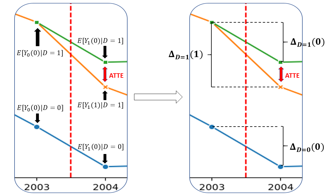
\[ \underbrace{\mathbb{E}[Y_{1}(0)|D=1] - \mathbb{E}[Y_{0}(0)|D=1] }_{=\Delta_{D=1}(0)}= \underbrace{\mathbb{E}[Y_{1}(0)|D=0] - \mathbb{E}[Y_{0}(0)|D=0]}_{=\Delta_{D=0}(0)} \]

Motivation

• The parameter of interest is the average treatment effect on the treated (ATTE)

\[ \theta_0:=\mathbb{E}[Y_{1}(1) - Y_{1}(0)| D=1] \]

• If the parallel trends assumptions is satisfied, the ATTE can be identified by

\[ \begin{align*} \theta_0: &= \underbrace{\Delta_{D=1}(1)}_{\text{Difference in treated}} - \underbrace{\Delta_{D=0}(0)}_{\text{Difference in untreated}} \end{align*} \]

• Presence of (pre-treatment) confounders: Conditional parallel trends

Identifying Assumptions

Conditional parallel trends:

\[ \mathbb{E}[Y_{1}(0) - Y_{0}(0)|X, D=1] = \mathbb{E}[Y_{1}(0) - Y_{0}(0)|X, D=0] \quad P-a.s. \]

No anticipation:

\[ \mathbb{E}[Y_{0}(0)|X, D=1] = \mathbb{E}[Y_{0}(1)|X, D=1] \quad P-a.s. \]

Overlap:

\[ \exists\epsilon > 0: P(D=1) > \epsilon \text{ and } P(D=1|X) \le 1-\epsilon \quad P-a.s. \] We also define \[ \begin{align*} \Delta Y_i &:= Y_{i1} - Y_{i0}\\ m(x) &:= P(D_i=1|X_i=x)\\ g(d,x) &:= \mathbb{E}[\Delta Y_i | D_i=d, X_i=x] \end{align*} \]

DML for DiD

Introduction to DML (Chernozhukov et al. 2018)

• Here: Panel data

• Score implemented as proposed in Chang (2020), Sant’Anna and Zhao (2020) and Zimmert (2018) \[ \psi(W,\theta,\eta) = -\frac{D}{p}\theta + \frac{D - m(X)}{p(1-m(X))}(Y_{1} - Y_{0}- g(0,X)) \] with \(\eta=(g, m, p)\).

• Nuisance components \[ \begin{align*} p_0 &= \mathbb{E}[D]\\ m_0(X) &= P(D=1|X)\\ g_0(0,X) &= \mathbb{E}[Y_{1} - Y_{0}|D=0, X] \end{align*} \]

DML for DiD

Introduction to DML (Chernozhukov et al. 2018)

• Why using DML for DiD?

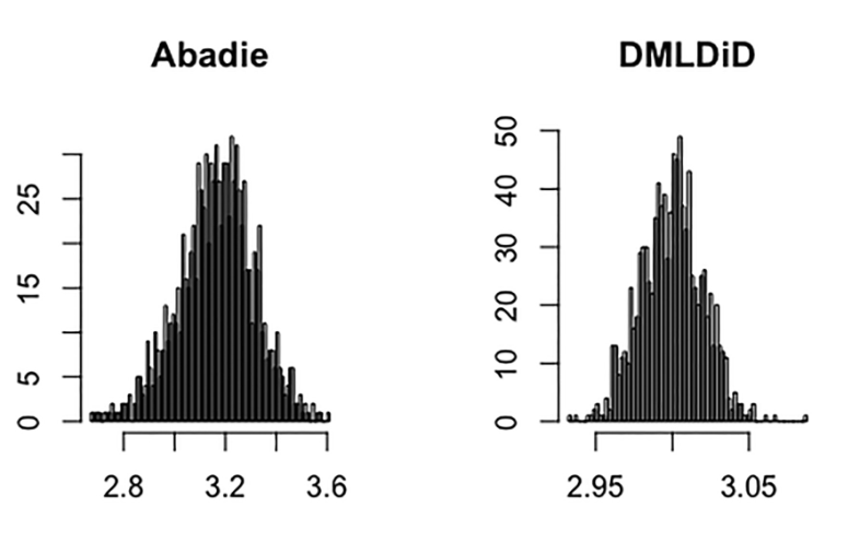
• Classical DiD estimators based on correct specification of propensity score or outcome regression (Sant’Anna and Zhao 2020)

• Shortcomings of TWFE

• Semiparametric estimators (Abadie 2005)

  • Not robust to regularization bias
  • Curse of dimensionality for classical nonparametric estimators

Source: Figure 1 of Chang (2020), \(\theta_0 = 3\).

DML for DiD

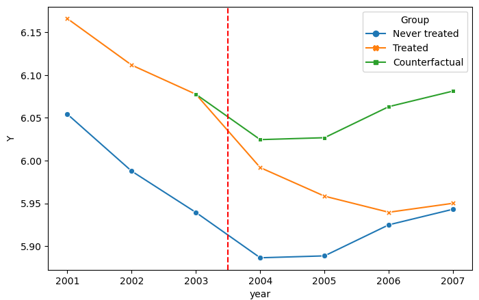
(Stylized) Example: Callaway and Sant’Anna (2021)

What is the causal effect of a minimum wage increase on youth unemployment?

• Here: 2 treatment groups (counties)

• Treatment: Increased minimum wage above federal minimum in 2003

DML for DiD

Estimation Example with DoubleML

import numpy as np
import pandas as pd
from doubleml import DoubleMLData
from doubleml import DoubleMLDID
from sklearn.ensemble import RandomForestRegressor, RandomForestClassifier
from sklearn.linear_model import LinearRegression, LogisticRegression
from sklearn.base import clone

# Load preprocessed data from URL 
df_subset = pd.read_csv("https://trainings.doubleml.org/trainings_materials/2024_march/courses/2023_dml_trainings/datasets/did_data/subset_did.csv")

# restrict to two time periods
df = df_subset.loc[(df_subset.year == 2003) | (df_subset.year==2004)].copy()
df.head(n=3)

def compute_difference(values):
    return values.iloc[1] - values.iloc[0]

df_diff = df.groupby("id").agg({"lpop": "first",
                                "lavg_pay": "first",
                                "region_2": "first",
                                "region_3": "first",
                                "region_4": "first",
                                "D": "first",
                                "Y": compute_difference}).reset_index()
df_diff.head(n=5)

# Prepare data backend
dml_data = DoubleMLData(df_diff, y_col="Y", d_cols="D",
                        x_cols=["lpop", "lavg_pay", "region_2", "region_3", "region_4"])
# print(dml_data)

# Initialize ML learners
ml_g = LinearRegression() #RandomForestRegressor()
ml_m = LogisticRegression() # RandomForestClassifier()

# Initialize DoubleMLDiD object
np.random.seed(42)
dml_did = DoubleMLDID(dml_data,
                      ml_g,
                      ml_m,
                      n_folds=50,
                      n_rep=1,
                      score='observational',
                      in_sample_normalization=True,
                      dml_procedure='dml2',
                      trimming_rule='truncate',
                      trimming_threshold=0.01)

dml_did.fit()

dml_did.summary

Sensitivity Analysis for Causal ML

Sensitivity Analysis for DML

What is Sensitivity Analysis?

• Sensitivity analysis is concerned with violations of underlying identification assumptions

• Classical example: Omitted (confounding) Variable Bias (OVB) for linear regression under conditional independence/exogeneity

• Cinelli and Hazlett (2020):

  • Strength of violation: How strong would a confounding relationship need to be in order to change the conclusions of our analysis?

  • Plausibility of violation: Would such a confounding relationship be plausibly present in our data?

Sensitivity Analysis for DML

What is Sensitivity Analysis?

• Strength of violations:
  • Define sensitivity parameters that reflect violations of the identification assumptions
• Compute OVB formula for each combination of these sensititivity parameters

• Linear regression (Cinelli and Hazlett 2020):
  • \(C_Y^2\): Partial \(R^2\) of \(Y\) with confounder \(U\), given we control for treatment \(D\) and observed confounders \(X\)
  • \(C_D^2\): Partial \(R^2\) of \(D\) with confounder \(U\), given we control for observed confounders \(X\)

import networkx as nx
import matplotlib.pyplot as plt

G = nx.DiGraph()

# Add nodes
G.add_node("D")
G.add_node("Y")
G.add_node("X")
G.add_node("U")
G.add_edge("D", "Y")
G.add_edge("X", "Y")
G.add_edge("X", "D")
G.add_edge("U", "D")
G.add_edge("U", "Y")

# Draw the graph
plt.figure(figsize=(4, 3)) 
pos = {"D": (0, 0), "Y": (2, 0), "X": (1,1), "U": (1,-1)}
edge_colors = ['black', 'black', 'black', 'red', 'blue']
nx.draw(G, pos, with_labels=True, node_size=800, node_color='lightblue',
 edge_color=edge_colors)
plt.show()

Sensitivity Analysis for DML

Sensitivity Analysis for DML

• Substantial generalization of sensitivity analysis in long story short approach (Chernozhukov et al. 2022) based on so-called Riesz Representation \[ \theta_0 = \mathbb{E}[m(W,g_0)] = \mathbb{E}[g_0(W)\alpha_0(W)], \] with \(g_0(W)\) referring to some form of a main outcome regression (\(Y\) on \(D\) and \(X\)) and \(\alpha_0(W)\) is the Riesz Representer

• In some sense, \(\alpha_0(W)\) implements the orthogonal moment condition required for DML, e.g., Frisch-Waugh-Lovel partialling out, doubly robust score for ATET or DiD

Introductory survey paper available soon: Bach, Chernozhukov, et al. (2024). Also see the Riesz Representer for FWL-style partially linear regression in Appendix 1.

Sensitivity Analysis for DML

Sensitivity Analysis for DML

• General bound on bias: \[ \text{bias}(\theta_s, \theta_0)^2 \leq \mathbb{E}\big[ (g_0-g_s)^2\big]\mathbb{E}\big[(\alpha_0-\alpha_s)^2 \big] = S^2 C_Y^2 C_D^2, \] where \(\theta_s\) is the short (=feasible) causal estimate and \(\theta_0\) the long (=true) parameter

• It is possible to express the bias in terms of the sensitivity parameters

• Exact formulation of \(C_Y^2\) and \(C_D^2\) depends on the causal model and estimate of interest (Cinelli and Hazlett (2020) as a special case for ATE in linear regression model)

Sensitivity Analysis for Difference-in-Difference Models

Sensitivity Analysis for DiD

Sensitivity Analysis for DiD

• Previous work on sensitivity analysis for DiD: Rambachan and Roth (2023), Manski and Pepper (2018), see sensitivity chapters Roth et al. (2023) ann Callaway (2023)

• Rambachan and Roth (2023): Make statements on DiD estimates based on PT violations from pretesting and/or under additional functional form assumptions

• Here: Extend long story short approach to DiD models

• Consider the 2x2 Panel Data Setting, the Identification Assumptions, and the Doubly Robust DiD Model from before

Sensitivity Analysis for DiD

Sensitivity Analysis for DiD

• Long form of the DiD model: PT holds conditional on \((X, U)\)

\[ \mathbb{E}[Y_{1}(0) - Y_{0}(0)|X, U, D=1] = \mathbb{E}[Y_{1}(0) - Y_{0}(0)|X, U, D=0] \quad P-a.s. \]

• However, with available data we can only estimate ATET based on the short model

\[ \mathbb{E}[Y_{1}(0) - Y_{0}(0)|X, D=1] = \mathbb{E}[Y_{1}(0) - Y_{0}(0)|X, D=0] \quad P-a.s. \]

• Question: How robust are the DiD estimates to violations of (conditional) PT?

Sensitivity Analysis for DiD

Sensitivity Analysis for DiD

• Riesz representation for DML DiD (with in-sample normalization)

\[ \begin{align}\begin{aligned}m(W,g) &= \big(g(1,X) - g(0,X))\frac{D}{\mathbb{E}[D]}\\\alpha(W) &= \frac{D}{\mathbb{E}[D]} - \frac{m(X)(1-D)}{\mathbb{E}[D](1-m(X))}.\end{aligned}\end{align}, \] with

\[ \begin{align*} m_0(X) &= P(D=1|X)\\ g_0(d,X) &= \mathbb{E}[Y_{1} - Y_{0}|D=d, X] = \mathbb{E}[\Delta Y | D=d, X] \end{align*} \]

Sensitivity Analysis for DiD

Sensitivity Parameters

\[ \begin{align} C^2_{\Delta Y} = R^2_{\Delta Y -g_s\sim g-g_s} = \frac{\mathrm{Var}\big(\mathbb{E}[\Delta Y|D, X, U]\big) - \mathrm{Var}\big(\mathbb{E}[\Delta Y|D, X]\big)}{\mathrm{Var}\big(\Delta Y\big) - \mathrm{Var}\big(\mathbb{E}[\Delta Y|D, X]\big)}, \end{align} \qquad(1)\] which measures the proportion or residual variance in the differenced outcomes \(\Delta Y\) explained by one or several unobserved (time-varying) confounders \(U\).

\[ \begin{align*} C_D^2= \frac{\mathbb{E}\left[\frac{m(X, U)}{1-m(X,U)}\right] - \mathbb{E}\left[\frac{m(X)}{1-m(X)}\right]}{\mathbb{E}\left[\frac{m(X)}{1-m(X)}\right]}, \end{align*} \qquad(2)\] which is the relative gain in average treatment probability ratio.

Sensitivity Analysis for DiD

Benchmarking

• We can plug in various values for \(C_D^2\) and \(C_Y^2\) to compute the bias on the ATET in scenarios of different violation strengths ➡️ Bias bounds, Contour plot

• Benchmarking: Relate these values to the context of the empirical analysis

• Idea: Mimic a situation of PT violation by leaving out one or several observed confounders from the causal model

• Example: Conditional PT vs. unconditional PT

Sensitivity Analysis for DiD

Example revisited

dml_did.sensitivity_analysis()

print(dml_did.sensitivity_summary)

Sensitivity Analysis for DiD

Example revisited: Benchmarking

• Recompute sensitivity parameters (gain statistics) by omitting all pre-treatment covariates (= comparison to unconditional PT )

from doubleml.utils import gain_statistics
df_bench = df_diff.loc[:,['D', 'Y']]
df_bench['const'] = 1

dml_data_bench = DoubleMLData(df_bench, y_col="Y", d_cols="D",
                        x_cols=["const"])
# print(dml_data)

# Initialize ML learners
ml_g = LinearRegression()
ml_m = LogisticRegression(penalty=None)

np.random.seed(42)
dml_did_bench = DoubleMLDID(dml_data_bench,
                      ml_g,
                      ml_m,
                      n_folds=50,
                      n_rep=1,
                      score='observational',
                      in_sample_normalization=True,
                      dml_procedure='dml2',
                      trimming_rule='truncate',
                      trimming_threshold=0.01)

dml_did_bench.fit()

dml_did_bench.sensitivity_analysis()

gain_stats_bench = gain_statistics(dml_did, dml_did_bench)
gain_stats_df = pd.DataFrame(gain_stats_bench)
gain_stats_df

• We find that the pre-treatment variables seem to have a strong predictive power for the treatment status but not for the outcome difference \(\Delta Y\)

Sensitivity Analysis for DiD

Example revisited: Contour Plot

dml_did.sensitivity_analysis(cf_d = gain_stats_bench['cf_d'][0], cf_y = gain_stats_bench['cf_y'][0], rho = gain_stats_bench['rho'][0])
dml_did.sensitivity_plot(grid_bounds=(0.32, 0.32))

Outlook and Challenges

Outlook and Challenges

• Conceptualization: Sensitivity for PT violations

• Relation to pre-testing and sensitivity analysis of Rambachan and Roth (2023)

• Extension to multi-treatment periods (Callaway and Sant’Anna 2021), GATET aggregation, reporting

• Application and evaluation based on various empirical studies

• Practical guidance and recommendations

Questions? Comments?

Thank you for your attention! 🙏

Appendix

Appendix 1: Double Machine Learning

• Motivation example: Partially linear regression model \[\begin{align*} Y & = D \theta_0 + g_0(X) + \zeta, & &\mathbb{E}[\zeta | D,X] = 0, \\ \end{align*} \qquad(3)\] with \(g_0()\) being a possibly non-linear function of high-dimensional covariates \(X\)

• Idea: Use ML-estimators to estimate \(g_0(X)\)
  • Lasso, Ridge, Elastic Net, Random Forests, Gradient Boosting, \(\ldots\)

Problem: Regularization bias from using ML-estimators

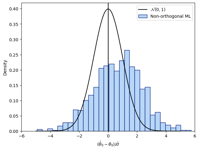
Empiricial distribution of naive ML-based estimator in a simulated data example (Chernozhukov et al. 2018).

Appendix 1: Double Machine Learning

Naive ML-Based Estimation Approach (Example)

1. Use ML to predict \(Y\) based on \(X\)

2. Plug in the ML predictions for \(Y\) for \(g(X)\) into Equation 3 and estimate linear regression

3. Use standard inference on the resulting coeficient estimate on \(\theta_0\) (\(t\)-tests, confidence intervals, \(p\)-values)

⚡ Problem: Regularization bias will generally lead to inconsistent estimation of \(\theta_0\) and non-normal asymptotic distribution of the naive estimator

Empiricial distribution of naive ML-based estimator in a simulated data example (Chernozhukov et al. 2018).

Neyman Orthogonality: Partialling Out

Partialling Out (Frisch-Waugh-Lovell Theorem)

1. Predict \(Y\) by \(\mathbb{E}[Y|X]\) using ML, save the residuals \(W\)

2. Predict \(D\) by \(\mathbb{E}[D|X]\) using ML, save the residuals \(V\)

3. Use linear regression of \(W\) on \(V\) to estimate \(\theta_0\)

4. Use standard inference for OLS (\(t\)-tests, confidence intervals, \(p\)-values)

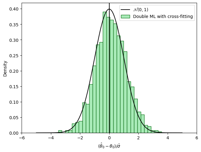
✅ Partialling out implements a Neyman-orthogonal moment condition

Empirical distribution of DML estimator in a simulated data example (Chernozhukov et al. 2018).

Appendix 1: Double Machine Learning

Neyman Orthogonality Example: Partialling Out

Technically, the inference framework is built on a moment condition that satisfies the property of Neyman orthogonality, i.e.,

\[\mathbb{E}[\underbrace{\psi(W; \theta_0, \eta_0)}_{\text{score function}}] = 0,\] with \(W\) denoting the data, \(\theta_0\) the causal parameter of interest (ATE), and \(\eta\) the nuisance part.

Neyman orthogonality ensures that the moment condition identifying \(\theta_0\) is insensitive to small pertubations of the nuisance function \(\eta\) around \(\eta_0\)

\[\left.\partial_\eta \mathbb{E}[\psi(W; \theta_0, \eta)] \right|_{\eta=\eta_0} = 0.\]

Appendix 1: Double Machine Learning

Neyman Orthogonality

The naive approach minimizes the following MSE \[ \begin{align}\small \min_{\theta} \mathbb{E}[(Y - D\theta - g_0(X))^2] \end{align} \]

Whereas for the partialling-out approach minimizes \[ \begin{align}\small \min_{\theta} \mathbb{E}\big[\big(Y - \mathbb{E}[Y|X] - (D-\mathbb{E}[D|X])\theta\big)^2\big] \end{align} \]

This implies the following moment equations

\[ \begin{align}\small \mathbb{E}[\underbrace{(Y - D\theta_0 - g_0(X))D}_{=:\psi (W, \theta_0, \eta_0)}]&=0 \end{align} \]

\[ \scriptsize \begin{align} \mathbb{E}\big[\underbrace{\big(Y - \mathbb{E}[Y|X] - (D-\mathbb{E}[D|X])\theta_0\big)(D-\mathbb{E}[D|X])}_{=:\psi (W, \theta_0, \eta_0)}\big]&=0 \end{align} \]

Neyman Orthogonality

Naive approach

\[ \small \begin{align} \psi (W, \theta_0, \eta_0) = & (Y - D\theta_0 - g_0(X))D \end{align} \]

FWL partialling out (Neyman orthogonal)

\[ \scriptsize \begin{align} \psi (W, \theta_0, \eta_0) = & \Big((Y- E[Y|X]) -(D-E[D|X])\theta_0\Big)\\ & (D-E[D|X]) \end{align} \]

With nuisance function \(\eta\) \[ \small \begin{align} \eta &= g(X), \\ \eta_0 &= g_0(X). \end{align} \]

With nuisance function \(\eta\) \[ \small \begin{align} \eta &= (\ell(X), m(X)), \\ \eta_0 &= ( \ell_0(X), m_0(X)), \\ &= ( \mathbb{E} [Y \mid X], \mathbb{E}[D \mid X]). \end{align} \]

Appendix 1: Double Machine Learning

High-Quality Machine Learning Estimators: PLR

• The nuisance parameters are estimated with high-quality (fast-enough converging) machine learning methods

• Chernozhukov et al. (2018): Different structural assumptions lead to the use of different machine-learning tools for estimating \(\eta_0\)

  • Example: Sparsity \(\rightarrow\) \(\ell_1\) penalized learners like lasso
  • Rates for specific learners are available in the literature

• Formal requirements are specific to the causal model and orthogonal score
  • PLR, partialling out: \(\lVert \hat{m}_0 - m_0 \rVert_{P,2} \times \big( \lVert \hat{m}_0 - m_0 \rVert_{P,2} + \lVert \hat{\ell}_0 - \ell_0\rVert _{P,2}\big) \le \delta_N N^{-1/2}\)
  • IRM example, doubly robust score, ATE: \(\lVert \hat{m}_0 - m_0 \rVert_{P,2} \times \lVert \hat{\ell}_0 - \ell_0\rVert _{P,2} \le \delta_N N^{-1/2}\)

Appendix 1: Riesz Representer PLR

• Riesz represention for the PLR example from before

\[ \begin{align} g_0(W) &= \mathbb{E}[Y|D,X,U] = \theta_0 D + g_(X, U) \\ g_s(W) &= \mathbb{E}[Y|D,X] = \theta_0 D + g_s(X) \end{align} \]

\[ \begin{align}\begin{aligned}\alpha_s(W) &= \frac{D-\mathbb{E}[D|X]}{\mathbb{E}[(D-\mathbb{E}[D|X]^2)]}\\ \\ \alpha_0(W) &= \frac{D-\mathbb{E}[D|X,U]}{\mathbb{E}[(D-\mathbb{E}[D|X,U]^2)]}\end{aligned}\end{align} \]

References

References

Abadie, Alberto. 2005. “Semiparametric Difference-in-Differences Estimators.” The Review of Economic Studies 72 (1): 1–19.

Bach, Philipp, Victor Chernozhukov, Carlos Cinelli, Lin Jia, Sven Klaasen, Nils Skotara, and Martin Spindler. 2024. “Sensitivity Analysis for Causal Machine Learning – a Tutorial.”

Bach, Philipp, Sven Klaassen, Kueck Jannis, Mara Mattes, and Martin Spindler. 2024. “Double Machine Learning and Sensitivity Analysis for Difference in Differences Models.”

Callaway, Brantly. 2023. “Difference-in-Differences for Policy Evaluation.” Handbook of Labor, Human Resources and Population Economics, 1–61.

Callaway, Brantly, and Pedro HC Sant’Anna. 2021. “Difference-in-Differences with Multiple Time Periods.” Journal of Econometrics 225 (2): 200–230.

Chang, Neng-Chieh. 2020. “Double/Debiased Machine Learning for Difference-in-Differences Models.” The Econometrics Journal 23 (2): 177–91.

Chernozhukov, Victor, Denis Chetverikov, Mert Demirer, Esther Duflo, Christian Hansen, Whitney Newey, and James Robins. 2018. “Double/Debiased Machine Learning for Treatment and Structural Parameters.” The Econometrics Journal 21 (1): C1–68. https://onlinelibrary.wiley.com/doi/abs/10.1111/ectj.12097.

Chernozhukov, Victor, Carlos Cinelli, Whitney Newey, Amit Sharma, and Vasilis Syrgkanis. 2022. “Long Story Short: Omitted Variable Bias in Causal Machine Learning.” National Bureau of Economic Research.

Cinelli, Carlos, and Chad Hazlett. 2020. “Making Sense of Sensitivity: Extending Omitted Variable Bias.” Journal of the Royal Statistical Society Series B: Statistical Methodology 82 (1): 39–67.

Cunningham, Scott. 2021. Causal Inference: The Mixtape. Yale university press.

De Chaisemartin, Clément, and Xavier d’Haultfoeuille. 2023. “Two-Way Fixed Effects and Differences-in-Differences with Heterogeneous Treatment Effects: A Survey.” The Econometrics Journal 26 (3): C1–30.

Manski, Charles F, and John V Pepper. 2018. “How Do Right-to-Carry Laws Affect Crime Rates? Coping with Ambiguity Using Bounded-Variation Assumptions.” Review of Economics and Statistics 100 (2): 232–44.

Rambachan, Ashesh, and Jonathan Roth. 2023. “A More Credible Approach to Parallel Trends.” The Review of Economic Studies 90 (5): 2555–91. https://doi.org/10.1093/restud/rdad018.

Roth, Jonathan, Pedro HC Sant’Anna, Alyssa Bilinski, and John Poe. 2023. “What’s Trending in Difference-in-Differences? A Synthesis of the Recent Econometrics Literature.” Journal of Econometrics.

Sant’Anna, Pedro HC, and Jun Zhao. 2020. “Doubly Robust Difference-in-Differences Estimators.” Journal of Econometrics 219 (1): 101–22.

Zimmert, Michael. 2018. “Efficient Difference-in-Differences Estimation with High-Dimensional Common Trend Confounding.” arXiv Preprint arXiv:1809.01643.